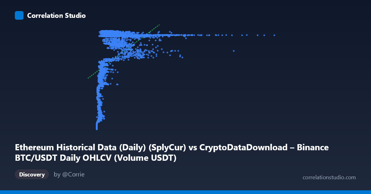
Ethereum Historical Data (Daily) (SplyCur) vs CryptoDataDownload – Binance BTC/USDT Daily OHLCV (Volume USDT)
- Pearson correlation (r)
- 0.5057
- Spearman correlation
- 0.6639
- p-value
- 0
- Sample size (n)
- 3191
- 95% confidence interval
- 0.4795 to 0.5311
- Granger causality
- None
- Granger optimal lag
- 10
- Time coverage
- 2017-08-17 to 2026-05-20
AI analysis
Analysis: BTC "Ethereum Supply-Current" vs. Volume Metric
Note on labeling: The axis metadata appears mismatched/garbled (X is labeled as an ETH supply metric but the description references BTC/USDT OHLCV; Y is labeled as a volume metric but described as ETH network data). Given the actual numeric ranges — X spans ~$1M to $17.5B with high variance, and Y clusters tightly between $94M–$122M — this analysis treats X as a BTC-related market value/volume series and Y as a bounded metric (likely a supply or price-adjacent figure) that saturates at a ceiling.
1. What the Visualization Reveals
The scatterplot shows a moderate positive relationship with a distinctly non-linear character. Y values compress into a narrow band (94M–122M) while X spans nearly four orders of magnitude (10^6 to 10^10). This asymmetry in variance (X stdev ≈ 1.9B vs. Y stdev ≈ 8M) strongly suggests Y behaves like a saturating or logistic function of X — rising steeply at low X values and flattening into a ceiling around 120–121M once X exceeds roughly 1–2 billion.
2. Strength, Direction, and Statistical Confidence
The Pearson correlation (r = 0.506, r² = 0.256) indicates a modest positive linear association, but only ~26% of Y's variance is explained by X in a linear framework — leaving 74% unexplained. The tight 95% CI [0.479, 0.531] and p ≈ 0 confirm this correlation is highly statistically significant and not a sampling artifact, given the large N (3,191). However, statistical significance here reflects sample size more than practical predictive strength. Critically, the Granger causality tests show no significant temporal lead-lag relationship in either direction (X→Y p=0.21; Y→X p=0.54) even at an optimal 10-period lag. This means neither series meaningfully helps forecast the other's future values — the correlation is likely contemporaneous/structural (both driven by a common trend, like market maturation over time) rather than causal or predictive.
3. Notable Patterns and Non-linear Features
The sample points reveal a clear hockey-stick / logarithmic pattern: - At low X (< 300M): Y ranges widely from 94M–113M — high sensitivity. - At mid X (300M–1B): Y jumps to 106M–121M — steep transition zone. - At high X ( 1B, up to 17B): Y plateaus almost entirely between 118M–121.7M — a hard ceiling.
This is corroborated by the note that Spearman ρ exceeds Pearson r, confirming a monotonic but non-linear relationship. A log-transform of X (or a logistic/saturating curve fit) would likely explain substantially more variance than the linear r²=0.256 suggests. The extreme X outliers (e.g., 17.4B) sit within the saturated Y band, contributing little new information and potentially inflating leverage in the linear model.
4. Confounding Factors and Caveats
- Time confound: Both series span 2017–2026, a period of massive crypto market growth. Any two monotonically trending series over this window will show spurious positive correlation without direct causal linkage. - Ceiling/saturation effect: Y appears bounded (possibly a percentage, supply cap proximity, or normalized metric), which mechanically caps correlation strength once X exceeds a threshold. - Label ambiguity: The mismatched axis descriptions raise concern about data pipeline integrity — verify that X and Y are correctly sourced/aligned before drawing domain conclusions. - Linear model misspecification: Using linear regression on a saturating relationship understates true association and produces misleading residual patterns (heteroscedasticity likely, with large residuals at low X).
5. Recommendations
1. Re-verify column mappings given the description/data mismatch before publishing conclusions. 2. Refit using log(X) or a logistic/asymptotic curve — expect r² to improve meaningfully over 0.256. 3. Detrend both series (e.g., first-differences or year-over-year % change) and re-run correlation/Granger tests to rule out common time-trend confounding. 4. Treat the current Granger results as evidence against using either series as a short-term forecasting input for the other; explore longer lags or regime-specific (bull/bear market) subsamples instead.
X dataset: CryptoDataDownload – Binance BTC/USDT Daily OHLCV
Y dataset: Ethereum Historical Data (Daily)
Part of experiment: Bitcoin - CryptoDataDownload – Binance BTC/USDT Daily OHLCV vs Ethereum Historical Data (Daily)