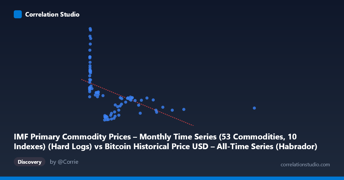
IMF Primary Commodity Prices – Monthly Time Series (53 Commodities, 10 Indexes) (Hard Logs) vs Bitcoin Historical Price USD – All-Time Series (Habrador) (Price)
- Pearson correlation (r)
- -0.5004
- Spearman correlation
- -0.6861
- p-value
- 0.000001
- Sample size (n)
- 83
- 95% confidence interval
- -0.6463 to -0.3191
- Granger causality
- None
- Granger optimal lag
- 10
AI analysis
Analysis: Bitcoin Price vs. IMF Commodity Price Index
1. What the Visualization Reveals
The scatterplot displays a clear inverse, curvilinear relationship rather than a clean linear one. At low X-values (roughly 0–500, likely early Bitcoin prices in USD), Y-values (commodity index) are highly dispersed, ranging from ~240 to ~453. As X increases beyond ~600–2450, the Y-values compress into a narrow, low band (roughly 255–295). This produces a pattern that resembles a decaying curve or hyperbola rather than a straight line — consistent with the note that Spearman's ρ exceeds Pearson's r.
2. Strength, Direction, and Statistical Confidence
The Pearson correlation (r = -0.50) indicates a moderate negative linear relationship, with r² = 0.25 meaning only 25% of the variance in the commodity index is explained by Bitcoin price (or vice versa) under a linear model — leaving 75% unexplained. The 95% CI [-0.646, -0.319] is reasonably tight and excludes zero, and the p-value (1.46×10⁻⁶) confirms this correlation is highly unlikely due to chance. However, statistical significance ≠ practical strength or causation. Critically, the Granger causality tests show no significant predictive direction in either direction (X→Y: p=0.896; Y→X: p=0.542), meaning neither series reliably forecasts the other over time — this is likely a contemporaneous/structural association rather than a causal lead-lag relationship.
3. Notable Patterns and Outliers
- Early-period clustering: Many points cluster at very low X (X<20) with high Y-variance (294 to 453) — this is the noisy, early Bitcoin era paired against a wide range of commodity index values. - High-X tail: A sparse but important cluster of points (X600) shows Y consistently compressed near 255–295, suggesting that once Bitcoin/X exceeds a threshold, the commodity index stabilizes in a narrower range. - Extreme outliers: Points like (8.21, 453.63), (13.09, 450.03), and (15.40, 430.49) — very low X but very high Y — pull the linear fit and inflate variance, while (2452.18, 268.39) is a lone high-leverage point on the X extreme. - The overall shape suggests a logarithmic or power-law decay fits better than a straight line, matching the Spearman/Pearson divergence noted.
4. Confounding Factors and Caveats
This is a time-series correlation problem in disguise — both variables are indexed to calendar time (2010–2017), so the negative correlation may simply reflect that Bitcoin price and the commodity index both evolved (in opposite general directions) over this period due to independent macro trends (Bitcoin's speculative growth vs. commodity price cycles), not a direct economic relationship. Additional concerns: - Non-stationarity: Both series likely trend over time, which can create spurious correlations. - Uneven sampling: Bitcoin's exponential price growth means early low-price points dominate the sample, skewing the linear fit. - Small n relative to population (83 of 449), raising sampling representativeness concerns. - Lack of Granger causality strongly implies any correlation is coincidental or driven by shared/external factors (e.g., global liquidity, USD strength, risk sentiment) rather than one series driving the other.
5. Actionable Insights
- Refit with a non-linear model (log-log or power law) given X's extreme right-skew (mean 321, max 2452) and the Spearman/Pearson divergence — this will likely improve explained variance substantially. - Log-transform X (as the column name "Hard Logs" suggests was possibly intended) before correlating, and re-run Granger tests on detrended/differenced series to check for spurious trend-driven correlation. - Control for time trend explicitly (e.g., include a time variable or use first-differences) to isolate whether the relationship holds beyond mutual drift. - Given no Granger causality, avoid using one series to forecast the other; instead investigate shared external drivers (USD index, global risk appetite, monetary policy) as a more productive research direction.
X dataset: Bitcoin Historical Price USD – All-Time Series (Habrador)
Y dataset: IMF Primary Commodity Prices – Monthly Time Series (53 Commodities, 10 Indexes)
Part of experiment: Bitcoin - Bitcoin Historical Price USD – All-Time Series (Habrador) vs IMF Primary Commodity Prices – Monthly Time Series (53 Commodities, 10 Indexes)