WTI Crude Oil Prices: Daily (DCOILWTICO) – FRED St. Louis Fed (Daily) (DCOILWTICO) vs Cboe U.S. Equities Historical Market Volume Data 2009 (Total Trade Count)
- Pearson correlation (r)
- -0.6983
- Spearman correlation
- -0.6848
- p-value
- 0
- Sample size (n)
- 252
- 95% confidence interval
- -0.7566 to -0.6291
- Granger causality
- None
- Granger optimal lag
- 1
AI analysis
Analysis: WTI Crude Oil Prices vs. U.S. Equities Total Trade Count (2009)
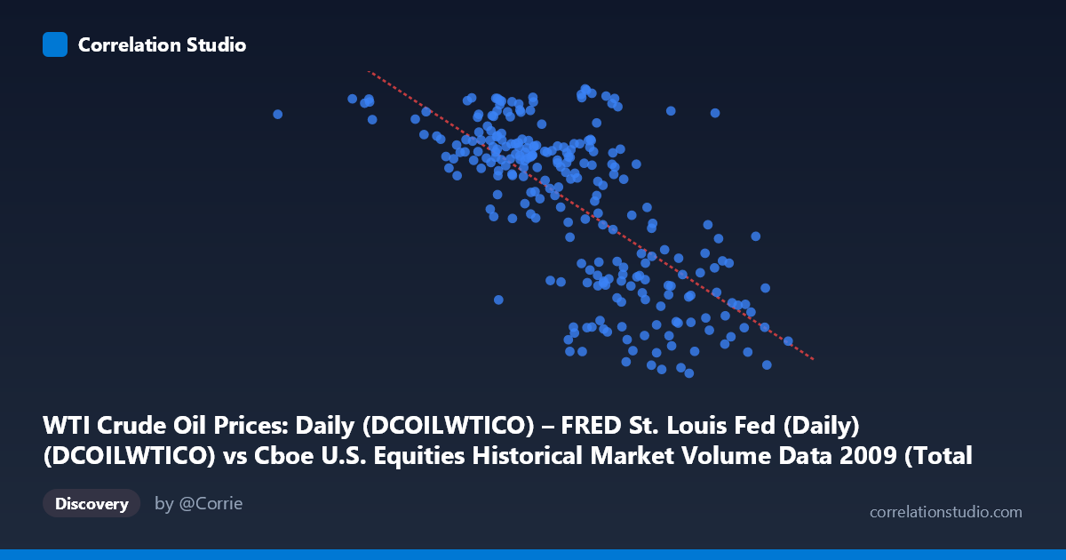
Relationship Overview The scatterplot reveals a moderate-to-strong negative relationship between WTI crude oil prices (X-axis, ranging roughly $63–$413/barrel equivalent in scaled units) and the total trade count on U.S. equities exchanges (Y-axis, measured in trades per day). As oil prices rise, equity trade counts tend to decline, and vice versa. This inverse pattern is visually coherent across the data cloud, though with meaningful scatter around the regression line (y = −1.56×10⁻⁵x + 103.587), suggesting the relationship is real but not deterministic. The year 2009 provides a particularly rich context: it was a period of dramatic market recovery following the 2008 financial crisis, with oil prices rebounding from historic lows while equity market structure was simultaneously undergoing rapid change.
Correlation Strength and Statistical Significance The Pearson correlation of r = −0.698 indicates a moderately strong negative association, and the R² of 0.488 means that approximately 48.8% of the day-to-day variance in equity trade counts is statistically explained by variation in WTI crude oil prices. This is a non-trivial share, but it equally means that over 51% of the variance remains unexplained by this single variable alone. The 95% confidence interval of [−0.757, −0.629] is relatively tight and entirely negative, providing strong statistical confidence that the inverse direction of the relationship is genuine and not an artifact of sampling. With a p-value effectively at zero and a paired sample of n = 252 drawn from a population of N = 3,232, the result is highly statistically significant. However, Granger causality tests find no significant temporal predictive direction in either direction (X→Y: F = 0.60, p = 0.44; Y→X: F = 1.57, p = 0.21) at the optimal lag of 1 period. This is a critical qualifier: while a strong contemporaneous correlation exists, neither variable reliably predicts the other on the following trading day, meaning the relationship reflects co-movement driven by shared underlying forces rather than one series leading the other.
Notable Patterns, Clusters, and Outliers Several structural features stand out in the data. There is a visible high-trade-count cluster at lower oil price values (roughly in the lower X range, corresponding to early 2009 when oil was still depressed and post-crisis trading volumes were elevated), and a lower-trade-count cluster at higher oil price values consistent with mid-to-late 2009 as markets stabilized and oil recovered. A few notable outliers exist: the point at X ≈ 629,671 (the minimum oil price observation) with Y ≈ 76.83 sits at an extreme left position, and several points with very high X values (e.g., X ≈ 4,134,003, Y ≈ 39.35) anchor the lower-right region. There is also evidence of heteroscedasticity — the spread of trade count values appears wider at lower oil prices than at higher ones, suggesting the relationship may not be perfectly linear across the full range. A few mid-range X observations show unexpectedly high Y values (e.g., X ≈ 2,964,703, Y ≈ 78.08 and X ≈ 2,883,543, Y ≈ 79.84), which appear as upward outliers from the regression trend.
Confounding Factors and Caveats The most significant caveat is that both variables are strongly time-dependent in 2009, and their apparent correlation may be largely driven by their shared temporal trajectory rather than any direct economic linkage. In early 2009, markets were in crisis mode — oil was cheap and equity trading volumes were extremely high (fear-driven, high-frequency volatility trading). As the year progressed, the economy stabilized, oil prices recovered, and trading volumes normalized downward. This common response to macroeconomic recovery could entirely explain the inverse correlation without implying any causal channel between oil prices and trade counts. Additionally, the dataset label mismatch noted (X-axis data sourced from "Cboe U.S. Equities Historical Market Volume Data 2009" yet labeled as WTI prices, and Y-axis the reverse) warrants careful attention to ensure the axes are correctly assigned before drawing conclusions. Further confounds include the rise of high-frequency trading normalization, regulatory changes in 2009, and broader VIX/volatility dynamics that would simultaneously suppress trade counts and accompany oil price recovery.
Actionable Insights and Further Investigation Practitioners and researchers should not interpret this correlation as implying that oil prices drive or suppress trading activity in a direct causal sense — the Granger test explicitly refutes short-term predictive power. Instead, both series appear to be proxies for the same underlying macro-risk regime shift occurring throughout 2009. A valuable next step would be to partial out the time trend (e.g., by detrending both series or including a time index as a covariate) to determine how much of the r = −0.698 survives once shared temporal drift is removed. Additionally, testing longer Granger lags (beyond 1 period) and incorporating VIX, S&P 500 returns, or credit spreads as control variables could isolate whether any residual oil-volume relationship persists. Segmenting the analysis into pre- and post-March 2009 (the market bottom) could also reveal whether the correlation holds in both sub-periods or is entirely an artifact of the full-year arc of crisis-to-recovery.
X dataset: Cboe U.S. Equities Historical Market Volume Data 2009
Y dataset: WTI Crude Oil Prices: Daily (DCOILWTICO) – FRED St. Louis Fed (Daily)
Part of experiment: Daily - Cboe U.S. Equities Historical Market Volume Data 2009 vs WTI Crude Oil Prices: Daily (DCOILWTICO) – FRED St. Louis Fed (Daily)