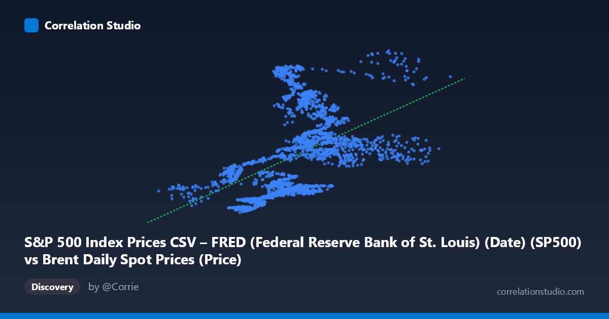
S&P 500 Index Prices CSV – FRED (Federal Reserve Bank of St. Louis) (Date) (SP500) vs Brent Daily Spot Prices (Price)
- Pearson correlation (r)
- 0.4795
- Spearman correlation
- 0.5862
- p-value
- 0
- Sample size (n)
- 2475
- 95% confidence interval
- 0.4485 to 0.5093
- Granger causality
- None
- Granger optimal lag
- 9
AI analysis
Analysis: Brent Crude Oil Prices vs. S&P 500 Index (2016–2026)
1. Overall Relationship Revealed
The scatterplot reveals a positive but loosely distributed relationship between daily Brent crude oil spot prices (X-axis, USD/barrel) and the S&P 500 index (Y-axis). As oil prices rise from roughly $10–$140/barrel, S&P 500 values tend to drift upward from approximately $2,000 to $7,500. However, the scatter is notably wide throughout the entire X range — at virtually any given oil price level, S&P 500 values span thousands of index points — indicating that oil price alone is a weak predictor of equity market levels. The linear regression (y = 34.87x + 1,515.34) captures the general directional trend but clearly misses substantial variation, and the hint that Spearman ρ exceeds Pearson r flags that the true underlying relationship is likely non-linear or driven by rank-order patterns rather than a clean linear mechanism.
2. Correlation Strength, Direction, and Causality
The Pearson correlation of r = 0.4795 indicates a moderate positive association, but the coefficient of determination tells a more sobering story: R² = 0.2299, meaning linear variation in Brent prices explains only about 23% of the variance in the S&P 500. The remaining ~77% is attributable to other factors entirely. The 95% confidence interval [0.4485, 0.5093] is relatively tight given the large sample (n = 2,475), and the p-value of effectively zero confirms this correlation is statistically real and not a sampling artifact. Crucially, however, the Granger causality tests find no significant predictive direction in either direction — neither X→Y (F = 1.557, p = 0.123) nor Y→X (F = 0.969, p = 0.464) — at the optimal lag of 9 periods. This is a critical finding: even though the two series are correlated in level, neither series temporally predicts the other. The correlation reflects co-movement likely driven by shared macro conditions rather than any causal mechanism.
3. Notable Patterns, Clusters, and Outliers
Several structural features stand out in the sample points. There is a dense cluster at lower oil prices (roughly $40–$75/barrel) paired with a wide range of S&P values ($2,000–$6,500), suggesting high equity market uncertainty independent of moderate oil prices — consistent with the COVID-era collapse and recovery period. A handful of high-oil-price observations (~$104–$138/barrel) correspond to mid-range S&P values (~$3,700–$4,600), arguably underperforming the regression line, which may reflect the 2022 energy shock when rising oil coincided with equity drawdowns. Conversely, several points at moderate oil prices ($67–$80) show very high S&P values ($5,500–$6,800), likely representing the 2024–2025 bull market. The observation at (119.03, 6,824.66) is particularly notable as an apparent high-leverage outlier combining elevated oil prices with record index levels. The Spearman ρ Pearson r discrepancy further suggests these extremes are distorting the linear fit.
4. Confounding Factors and Interpretive Caveats
This correlation is heavily susceptible to spurious co-movement driven by shared macroeconomic drivers. Both oil prices and equity markets respond to global growth expectations, Federal Reserve monetary policy, U.S. dollar strength, and geopolitical events — meaning their positive correlation may primarily reflect "risk-on / risk-off" cycles rather than any direct oil-equity mechanism. The time coverage (2016–2026) spans multiple distinct regimes: the 2020 COVID crash (oil went negative in futures; S&P plunged and recovered), the 2021–2022 inflationary surge, and the 2023–2025 AI-driven equity rally. These regime shifts create structural breaks that a single linear model cannot accommodate. Additionally, the axes appear to be mislabeled in the source data metadata (X is described as S&P dates but contains oil price values, and vice versa), which warrants careful verification before any operational use. Non-stationarity of both time series (both trend upward over time) may be artificially inflating the measured correlation.
5. Actionable Insights and Further Investigation
Given these findings, several next steps are warranted. First, detrend or difference both series (first differences or log returns) to remove shared upward time trends and test whether the correlation persists in stationary form — it likely weakens substantially. Second, fit a non-linear model (polynomial or logarithmic) as suggested by the Spearman/Pearson divergence, and test whether it meaningfully improves R² beyond the current 23%. Third, segment the analysis by macro regime (pre-COVID, COVID shock, inflationary period, post-2023) to determine whether the correlation is stable or regime-dependent. Fourth, consider incorporating a third variable such as the U.S. Dollar Index (DXY) or 10-year Treasury yields as a potential common driver explaining the co-movement. Finally, the absence of Granger causality at 9-period lags strongly argues against using oil prices as a tactical trading signal for S&P 500 direction — practitioners should not treat this moderate correlation as actionable for short-term forecasting.
X dataset: Brent Daily Spot Prices
Y dataset: S&P 500 Index Prices CSV – FRED (Federal Reserve Bank of St. Louis) (Date)
Part of experiment: Daily - Brent Daily Spot Prices vs S&P 500 Index Prices CSV – FRED (Federal Reserve Bank of St. Louis) (Date)