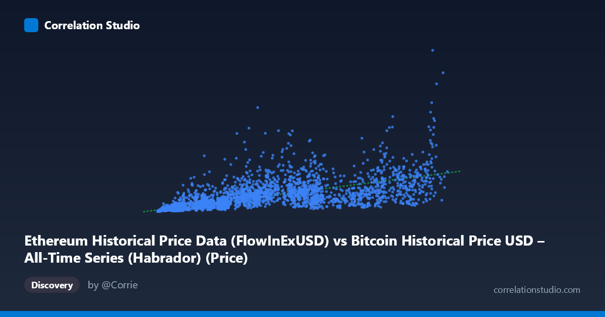
Ethereum Historical Price Data (FlowInExUSD) vs Bitcoin Historical Price USD – All-Time Series (Habrador) (Price)
- Pearson correlation (r)
- 0.7065
- Spearman correlation
- 0.893
- p-value
- 0
- Sample size (n)
- 3942
- 95% confidence interval
- 0.6905 to 0.7218
- Granger causality
- None
- Granger optimal lag
- 10
- Time coverage
- 2015-08-08 to 2026-05-23
- Recomputed on refreshed data
- 2026-10-24 (r was 0.7114)
AI analysis
Analysis: Ethereum "FlowInExUSD" vs. Bitcoin Historical Price (Mislabeled Series)
1. What the Visualization Reveals
Before interpreting the statistics, it's worth flagging a labeling oddity: the X-axis is described as an Ethereum flow metric while the Y-axis is labeled Bitcoin price, but the sample data shows X values in the hundreds-to-low-hundred-thousands and Y values ranging into billions — this pattern (small-to-mid X paired with a Y that spans ~5 orders of magnitude) is much more consistent with X representing Bitcoin price and Y representing Ethereum-related market cap or aggregate flow figures, or possibly the columns are simply swapped in the metadata. Regardless of labeling, the visualization shows a clear positive, monotonic relationship: as X increases, Y increases, but the growth in Y is disproportionate — small X values correspond to Y in the thousands, while large X values push Y into the billions, suggesting multiplicative/exponential rather than additive scaling.
2. Strength, Direction, and Uncertainty
The Pearson correlation of r = 0.7114 indicates a moderately strong positive linear relationship, with r² = 0.506 meaning the linear model explains just about half (50.6%) of the variance in Y — a substantial share, but leaving the other half unexplained by X alone. The tight 95% CI [0.6955, 0.7265] combined with p ≈ 0 confirms this correlation is highly statistically reliable given the large sample (n=3,917), not a product of chance. However, statistical significance here reflects sample size more than practical precision — with r² at ~0.5, X is a meaningful but incomplete predictor of Y. Critically, the Granger causality test shows no significant predictive direction in either direction (p = 0.19 and p = 0.26), meaning that despite the strong contemporaneous correlation, neither variable reliably leads the other in time. This strongly suggests the relationship is driven by a shared external factor (e.g., overall crypto market sentiment, macro liquidity cycles) rather than one asset causally driving the other's price with a lag.
3. Notable Patterns and Non-Linear Features
The data clearly exhibits heteroscedasticity and non-linear curvature: Y's range spans from ~16,766 to over 6.9 billion (5+ orders of magnitude) while X spans a much narrower ~600x range. Sample points show that at similar X values (e.g., ~9,000–10,000), Y varies wildly (from ~51 million to ~589 million), indicating substantial scatter/noise at any given X, especially in the low-to-mid X range. At the highest X values (100k+), Y still varies by an order of magnitude (219M to 6.9B), suggesting increasing variance at higher magnitudes — classic multiplicative/log-normal behavior. The note that Spearman ρ exceeds Pearson r confirms suspicion of non-linearity; a log-log or power-law transformation is likely far more appropriate than the current linear fit (y = 12942x + 5.69×10⁷), which will systematically underfit low-X, low-Y observations and overfit extreme values.
4. Confounding Factors and Caveats
Several caveats apply. First, crypto assets are notoriously co-integrated through common market beta — both BTC and ETH (or their derived metrics) respond similarly to macro liquidity, regulatory news, and speculative sentiment, producing spurious-looking correlation without direct causal linkage. Second, the extreme scale disparity in Y (16K to 6.9B) hints that Y may combine heterogeneous regimes (e.g., early-history low-volume days vs. mature high-cap days), which a single linear/global model cannot capture well — time-based regime shifts (bull/bear cycles from 2015–2026) likely dominate the variance more than the X variable itself. Third, the label confusion (as noted above) raises real concerns about data pipeline integrity — verify column-to-dataset mapping before drawing economic conclusions. Finally, daily crypto price/flow series are highly autocorrelated (trending), which can inflate simple Pearson/Spearman correlations even when Granger causality (which controls for autocorrelation) finds no genuine lead-lag relationship.
5. Recommendations for Further Investigation
1. Verify variable labeling — confirm which column truly represents Ethereum flow vs. Bitcoin price before publishing conclusions. 2. Apply log-log transformation to both axes and refit — given the order-of-magnitude spread and Spearman/Pearson divergence, a power-law (y = a·x^b) model will likely dramatically improve fit. 3. Segment by time period/market regime (bull vs. bear cycles) to see if the relationship is stable or driven by specific historical eras (e.g., 2017, 2021, 2024 bull runs). 4. Test cointegration (e.g., Engle-Granger or Johansen test) rather than simple Granger causality on levels, since both series are likely non-stationary trending price series — this is more appropriate for financial time series with common trends. 5. Introduce a control variable (e.g., total crypto market cap or a liquidity index) to test whether the X-Y correlation is spurious/confounded by shared macro drivers.
X dataset: Bitcoin Historical Price USD – All-Time Series (Habrador)
Y dataset: Ethereum Historical Price Data
Part of experiment: Bitcoin - Bitcoin Historical Price USD – All-Time Series (Habrador) vs Ethereum Historical Price Data