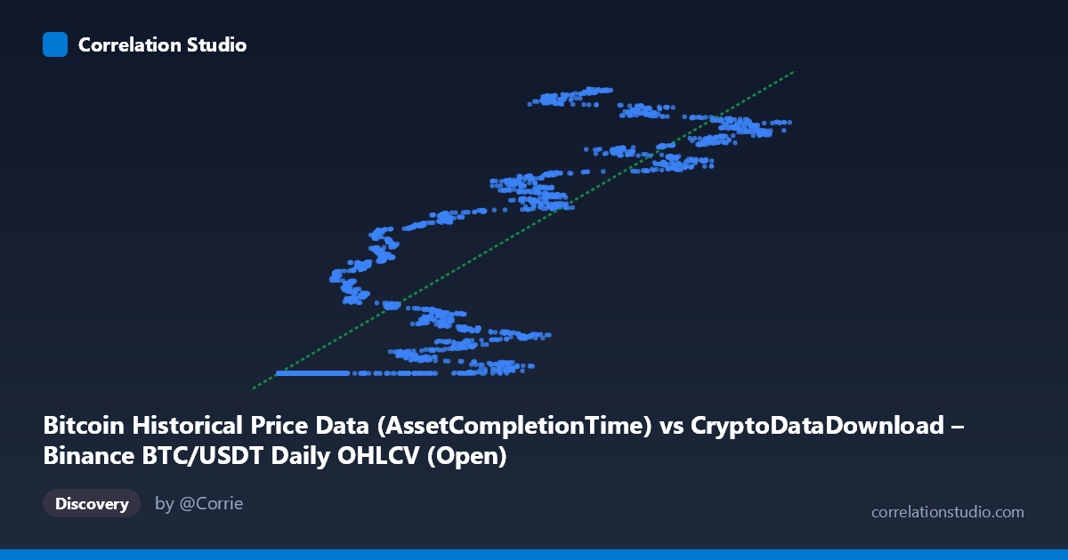
Bitcoin Historical Price Data (AssetCompletionTime) vs CryptoDataDownload – Binance BTC/USDT Daily OHLCV (Open)
- Pearson correlation (r)
- 0.8518
- Spearman correlation
- 0.8876
- p-value
- 0
- Sample size (n)
- 3191
- 95% confidence interval
- 0.842 to 0.8611
- Granger causality
- None
- Granger optimal lag
- 10
- Time coverage
- 2017-08-17 to 2026-05-20
AI analysis
Analysis: Bitcoin Historical Price Data vs. Binance BTC/USDT (AssetCompletionTime)
1. What the Visualization Reveals
This scatterplot is unusual in that it does not depict a relationship between two economically distinct variables — it plots "AssetCompletionTime" (a timestamp-like field, likely a record completion/processing indicator that scales with elapsed time or record index) against BTC/USDT opening prices drawn from what appears to be the same underlying dataset (Binance daily OHLCV), just packaged under two different dataset labels. The pattern that emerges is a step-like, non-linear curve: a long flat plateau near Y ≈ 1,614,337,000 for X values roughly below 20,000, followed by a steep, quasi-linear climb up to Y ≈ 1,779,000,000 as X increases beyond that threshold. This is characteristic of a cumulative or monotonically increasing series (e.g., a running timestamp or sequence counter) plotted against another increasing series (price growth over time), rather than two independently varying financial metrics.
2. Strength, Direction, and Statistical Confidence
The Pearson correlation of r = 0.852 (r² = 0.726) indicates a strong positive association, with the linear model explaining about 72.6% of the variance in Y. The 95% CI [0.842, 0.861] is tight, and the p-value of ~0 confirms the relationship is not due to chance at this sample size (n = 3,191). However, r² of 0.73 also means ~27% of the variance is not captured by the linear fit — consistent with the visible plateau-then-ramp shape, which a straight line fits only approximately. Critically, the Granger causality tests show no significant predictive direction in either direction (X→Y: p = 0.33; Y→X: p = 0.15) at the optimal lag of 10 periods. This means that despite the strong contemporaneous correlation, neither series is a statistically useful leading indicator of the other over time — the association is best interpreted as co-movement (likely both driven by the same underlying time/price trend) rather than one causing or forecasting the other.
3. Notable Patterns and Outliers
The most striking feature is the two-regime structure: a dense cluster of points where X < ~20,000 all map to a nearly constant Y (~1,614,337,000–1,614,338,000), suggesting these X values correspond to an early period (2017–~2019) when BTC price barely moved from its dataset's minimum baseline. Beyond X ≈ 20,000, Y increases steeply and almost linearly with X, reflecting Bitcoin's major price appreciation era. This is not a smooth linear relationship but a hockey-stick / threshold pattern, meaning a single linear regression (y = 1429.51x + 1.61e9) will systematically underfit the flat region and overfit the steep region — explaining why r² caps at 0.73 despite a visually strong trend. No extreme outliers are apparent beyond this structural bend; the "noise" band widens somewhat in the upper-X range (prices ranging ~1.71B–1.78B for similar X), indicating heteroscedasticity.
4. Confounding Factors and Caveats
The core caveat is that X is likely a disguised time proxy (an "AssetCompletionTime" field), not an independent causal variable — so this scatterplot may effectively be a time-series plot of BTC price relative to a monotonic index, mechanically producing high correlation without meaningful causal content. Both series may derive from overlapping or identical source data (Binance BTC/USDT OHLCV), risking data leakage/circularity — correlating a variable with a near-copy or transformation of itself inflates r spuriously. Additionally, financial time series like BTC price are non-stationary and trend-dominated, which commonly produces high correlations with any monotonically increasing series (e.g., record counts, timestamps, cumulative volume) — a classic spurious correlation risk. The lack of Granger causality further supports treating this as coincidental/structural co-trending rather than a genuine bivariate relationship.
5. Actionable Insights
Before drawing conclusions, clarify what "AssetCompletionTime" actually represents (raw timestamp, sequence ID, or derived metric) and confirm it is not a transformation of the same price series. If genuine time-series analysis is the goal, difference or detrend both series (e.g., use log returns instead of levels) and re-test correlation/Granger causality on stationary data — this will likely reveal whether any real short-term relationship exists once the shared trend is removed. Segmenting the analysis into the two visible regimes (pre-2019 flat period vs. post-2019 growth period) and fitting a piecewise or non-linear (e.g., logistic/exponential) model would better capture the true shape than a single linear fit. Finally, since Granger tests show no predictive edge either way, this pairing should not be used for forecasting purposes — instead, treat it as a data-quality/structure check on the two datasets' consistency.
X dataset: CryptoDataDownload – Binance BTC/USDT Daily OHLCV
Y dataset: Bitcoin Historical Price Data
Part of experiment: Bitcoin - CryptoDataDownload – Binance BTC/USDT Daily OHLCV vs Bitcoin Historical Price Data