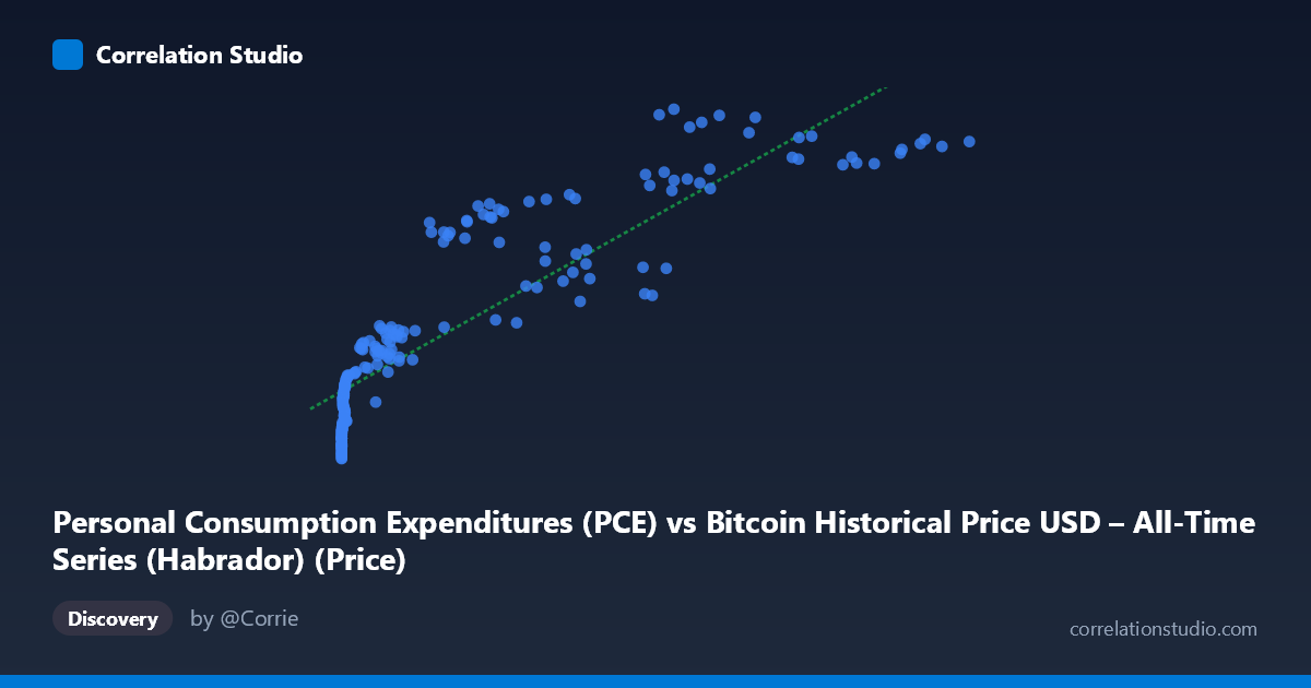
Personal Consumption Expenditures (PCE) vs Bitcoin Historical Price USD – All-Time Series (Habrador) (Price)
- Pearson correlation (r)
- 0.8843
- Spearman correlation
- 0.9696
- p-value
- 0
- Sample size (n)
- 193
- 95% confidence interval
- 0.8491 to 0.9116
- Granger causality
- None
- Granger optimal lag
- 10
- Time coverage
- 2010-08-01 to 2026-08-01
- Recomputed on refreshed data
- 2026-10-24 (r was 0.8799)
AI analysis
Analysis: Bitcoin Price vs. Personal Consumption Expenditures
1. Relationship Overview
The scatterplot reveals a strong, non-linear, monotonically increasing relationship between Bitcoin price (X) and PCE (Y). The shape is characteristic of a logarithmic or saturating curve rather than a straight line: Y rises steeply as X moves from near-zero to a few thousand dollars, then flattens considerably as X extends into the tens of thousands. This is confirmed by the data itself — X spans nearly six orders of magnitude (0.06 to 118,670), while Y varies only modestly (10,307 to 21,979), a range of roughly 2x. The linear regression (y = 0.0998x + 12,617) captures the broad trend but is clearly a poor structural fit given the extreme skew in X (mean 20,533, stdev 29,894 — heavily right-skewed).
2. Strength, Direction, and Statistical Confidence
The Pearson correlation (r = 0.88, r² = 0.775) indicates a strong positive linear association, with the linear model explaining about 77.5% of the variance in Y. The 95% CI [0.844, 0.909] is tight and excludes zero, and the p-value ≈ 0 confirms this correlation is highly unlikely to be due to chance in this sample. However, correlation strength should not be conflated with causal or predictive power: the Granger causality tests show no significant predictive relationship in either direction (X→Y: p=0.73; Y→X: p=0.63) even at an optimal lag of 10 periods. This means neither variable's past values help forecast the other's future values in a time-series sense — the strong r is likely driven by both series independently trending upward over the same historical period (2010–2026) rather than one causing or leading the other.
3. Notable Patterns and Outliers
Several features stand out: - Compressed low-X cluster: A large mass of points sits at X < 1,000 (early Bitcoin history) where Y ranges from ~10,700 to ~13,500 — showing that PCE grew substantially even while Bitcoin was worth pennies to a few hundred dollars. - Curvature/saturation: Above X ≈ 50,000, Y increases only slightly (16,000–22,000 range) despite X more than doubling, suggesting a log-linear rather than linear relationship — consistent with r² likely improving under a log(X) transformation. - High-X outliers: Points like (68,074, 21,979) and (86,473, 21,446) show some non-monotonic wobble — Y dips and rises without matching X's trajectory, hinting at independent macro cycles (COVID-era stimulus/inflation) affecting PCE separately from Bitcoin's price swings. - No true bivariate outliers: despite the extreme X range, points broadly hug the log-shaped trend, indicating the relationship, while nonlinear, is fairly consistent.
4. Confounding Factors and Caveats
This is a textbook case of spurious correlation via shared time trend. Both Bitcoin price and PCE have risen substantially from 2010–2026 due to entirely different underlying drivers — Bitcoin due to speculative adoption cycles and halving events, PCE due to population growth, inflation, and wage growth. Neither is mechanistically linked to the other. The lack of Granger causality strongly supports this interpretation: the correlation is likely an artifact of two non-stationary trending series sampled over the same calendar period, not evidence of any economic mechanism connecting Bitcoin prices to consumer spending. Additionally, monthly PCE (macro, smooth, low-frequency) is being compared to Bitcoin price (volatile, high-frequency), a scale/frequency mismatch that can distort naive correlation.
5. Suggested Further Investigation
- Detrend both series (e.g., first-difference or use year-over-year % change) before correlating, to test whether the relationship survives removing the common trend — this is the standard fix for spurious time-trend correlations. - Log-transform X given its extreme skew; refit regression as y ~ log(x) to check if r² improves and the relationship becomes more linear/interpretable. - Test stationarity (ADF/KPSS) on both series; if both are non-stationary and cointegration is absent, the relationship should not be interpreted as meaningful. - Treat this correlation as descriptive co-trending, not predictive or causal, per the Granger results — avoid using Bitcoin price as a leading indicator for PCE or vice versa in forecasting models.
X dataset: Bitcoin Historical Price USD – All-Time Series (Habrador)
Y dataset: Personal Consumption Expenditures
Part of experiment: Bitcoin - Bitcoin Historical Price USD – All-Time Series (Habrador) vs Personal Consumption Expenditures