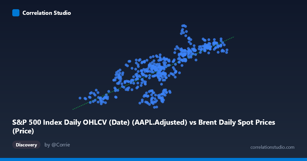
S&P 500 Index Daily OHLCV (Date) (AAPL.Adjusted) vs Brent Daily Spot Prices (Price)
- Pearson correlation (r)
- 0.76
- Spearman correlation
- 0.776
- p-value
- 0
- Sample size (n)
- 504
- 95% confidence interval
- 0.7204 to 0.7946
- Granger causality
- None
- Granger optimal lag
- 1
AI analysis
Scatterplot Analysis: AAPL Adjusted Price vs. Brent Crude Oil Spot Price (2015–2017)
1. Overall Relationship The scatterplot reveals a moderately strong positive relationship between AAPL's adjusted stock price (X-axis) and Brent crude oil spot prices (Y-axis) over the two-year period from February 2015 to February 2017. As AAPL's price increases, Brent crude prices tend to rise as well, following a generally upward-sloping linear trend described by the regression equation y = 0.934x + 65.35. The relationship is visually coherent across much of the range, though considerable vertical scatter around the regression line is evident, particularly in the mid-range X values (roughly 44–56), suggesting meaningful variability that the linear model does not fully capture.
2. Correlation Strength, Direction, and Causality The Pearson correlation of r = 0.76 indicates a strong positive association, and the R² of 0.578 means approximately 57.8% of the variance in Brent crude prices is statistically explained by AAPL's price movements — a substantial but far from complete explanation, leaving ~42% attributable to other factors. The 95% confidence interval of [0.72, 0.79] is relatively narrow, reflecting high precision given the large sample (n = 504), and the p-value of effectively zero confirms this correlation is statistically indistinguishable from chance. However, the Granger causality analysis tells a critically different story: neither direction of temporal prediction is significant (X→Y: F = 0.14, p = 0.71; Y→X: F = 0.64, p = 0.42). This means that despite the strong correlation, neither variable reliably predicts the other's future values — a crucial finding that strongly argues against any causal or directional interpretive framing.
3. Notable Patterns, Clusters, and Outliers Several structural features are visible in the data. There is a notable cluster of points in the 44–55 AAPL range with a wide vertical spread in Brent prices (~90–135), indicating high conditional variance at typical AAPL price levels. A few potential outliers stand out: the point near (54.16, 135.35) sits noticeably above the regression line, while points such as (46.08, 91.15) and (32.35, 92.07) fall well below it. The lower-left region (AAPL ~28–38, Brent ~89–108) appears relatively tightly clustered, while the upper-right (AAPL ~60–66, Brent ~120–126) shows moderate grouping — suggesting the relationship may be somewhat tighter at the extremes than in the middle range. A mild heteroscedastic pattern cannot be ruled out.
4. Confounding Factors and Interpretive Caveats The most significant caveat is that this correlation almost certainly reflects a common temporal driver rather than any meaningful economic link between AAPL stock and crude oil prices. Both series span 2015–2017, a period with distinct macroeconomic regimes: a global equity recovery, oil price collapse and partial recovery, and USD fluctuations. Shared time trends (non-stationarity) are the most likely source of spurious correlation — both variables may simply be co-moving with broader market sentiment, risk appetite, or global growth expectations. The dataset labeling also raises a metadata concern: the axes appear swapped in their dataset descriptions (AAPL data labeled under "Brent" dataset and vice versa), warranting verification. Additionally, with daily data, autocorrelation within each series can inflate apparent correlations and effectively reduce the true degrees of freedom well below n = 504.
5. Actionable Insights and Further Investigation Given the strong correlation but absent Granger causality, the immediate recommendation is to detrend or difference both series (e.g., use daily log-returns rather than price levels) before drawing any conclusions — this would remove shared trend artifacts and reveal whether any genuine co-movement exists at the short-term frequency. Further steps should include: (a) testing for cointegration to determine if a stable long-run equilibrium relationship exists; (b) examining residuals from the regression for autocorrelation patterns using Durbin-Watson or ACF/PACF plots; (c) introducing macroeconomic controls such as USD index, VIX, or global GDP proxies to assess whether the correlation disappears when confounders are included; and (d) verifying dataset alignment and labeling integrity, particularly the apparent axis-dataset mismatch noted above. As it stands, this correlation should be treated as a coincidental co-movement artifact of the specific time window rather than evidence of any economically meaningful relationship.
X dataset: Brent Daily Spot Prices
Y dataset: S&P 500 Index Daily OHLCV (Date)
Part of experiment: Daily - Brent Daily Spot Prices vs S&P 500 Index Daily OHLCV (Date)