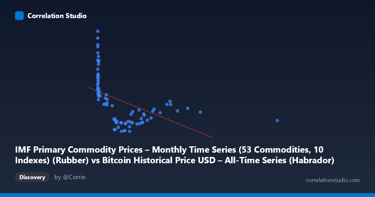
IMF Primary Commodity Prices – Monthly Time Series (53 Commodities, 10 Indexes) (Rubber) vs Bitcoin Historical Price USD – All-Time Series (Habrador) (Price)
- Pearson correlation (r)
- -0.4953
- Spearman correlation
- -0.7319
- p-value
- 0.000002
- Sample size (n)
- 83
- 95% confidence interval
- -0.6423 to -0.313
- Granger causality
- None
- Granger optimal lag
- 3
- Time coverage
- 2010-08-01 to 2017-06-01
- Recomputed on refreshed data
- 2026-10-24 (r was -0.4953)
AI analysis
Analysis: Rubber Prices vs. Bitcoin Price
1. Relationship Overview
The scatterplot displays a moderate negative association between rubber commodity prices (X-axis) and Bitcoin price (Y-axis). The data shows a clear non-linear pattern rather than a simple linear decline: at very low X-values (near 0, likely representing an early time period or data alignment artifact), Y-values are highest and most dispersed (ranging from ~130 to 280), while as X increases beyond ~100, Y-values compress into a much tighter band (roughly 55–140) and drift only slightly downward across the remaining range up to 2452. This suggests the relationship is driven heavily by a cluster of low-X points rather than a consistent trend across the full domain.
2. Strength, Direction, and Statistical Confidence
The Pearson correlation (r = -0.4953, R² = 0.245) indicates a moderate negative linear relationship, but only about 24.5% of the variance in Bitcoin price is explained by rubber price in this linear framing — leaving the majority (75%) unexplained by this single variable. The 95% CI [-0.642, -0.313] is reasonably tight and entirely negative, and the p-value (1.94E-06) confirms this correlation is statistically significant and not due to chance, despite the modest sample size (n=83 paired points from a population of 449). However, statistical significance should not be conflated with strong predictive power — R² of 0.245 is weak-to-moderate at best. Critically, Granger causality tests show no significant predictive direction in either direction (X→Y: p=0.474; Y→X: p=0.119), meaning neither variable reliably forecasts the other over time at the tested lag. This strongly suggests the correlation is either coincidental, driven by a shared underlying trend, or mediated by a confounding factor — not a genuine causal or lead-lag relationship.
3. Patterns, Clusters, and Outliers
The chart reveals at least two distinct regimes: (a) a cluster of low-X points (X < 20) with high, widely-scattered Y-values (up to 280.79), and (b) a much denser cluster spanning X from ~100 to 2452 with Y compressed near 55–140. This bimodal structure — rather than smooth linear decay — is consistent with the note that Spearman ρ exceeds Pearson r, indicating the true relationship is likely logarithmic or curvilinear (e.g., a steep early decline followed by a long, flat tail). The point at X=2452.18 (Y=79.77) is a notable high-leverage outlier that could disproportionately influence the linear fit. The extreme Y-values near X≈0 (e.g., Y=280.79, 265.49, 250.36) also warrant scrutiny as potential high-influence points.
4. Confounding Factors and Caveats
Both series are time-stamped (2010–2017), and Bitcoin's price history is dominated by exponential growth/bust cycles unrelated to commodity markets — meaning any correlation with rubber prices is more likely attributable to coincidental co-trending over time (both series evolving on their own timelines) rather than a genuine economic linkage. Since X and Y here appear to be mismatched/misaligned in the metadata (column labels are swapped between datasets), it's essential to verify that the temporal indexing between rubber prices and BTC price is correct and that both are sampled from the same calendar dates. Additionally, with only 83 paired samples drawn from 449 possible points, sampling method (every-nth selection) could introduce bias if the underlying data has cyclical or seasonal structure.
5. Recommendations for Further Investigation
Given the non-linear signal (Spearman Pearson) and the lack of Granger causality, I recommend: (1) re-fitting with a logarithmic or piecewise model to formally test whether a log(X) transformation improves fit substantially over the linear R²=0.245; (2) explicitly plotting the time series of both variables to check for spurious correlation from shared macro trends (e.g., both influenced by global liquidity/inflation in 2011 and 2013-2017); (3) testing Granger causality at multiple lag lengths (not just 3) given monthly data may have longer transmission lags; and (4) treating this correlation as descriptive/exploratory only — not a basis for trading or causal claims — until confounders (e.g., USD strength, global risk sentiment) are controlled for via multivariate analysis.
X dataset: Bitcoin Historical Price USD – All-Time Series (Habrador)
Y dataset: IMF Primary Commodity Prices – Monthly Time Series (53 Commodities, 10 Indexes)
Part of experiment: Bitcoin - Bitcoin Historical Price USD – All-Time Series (Habrador) vs IMF Primary Commodity Prices – Monthly Time Series (53 Commodities, 10 Indexes)