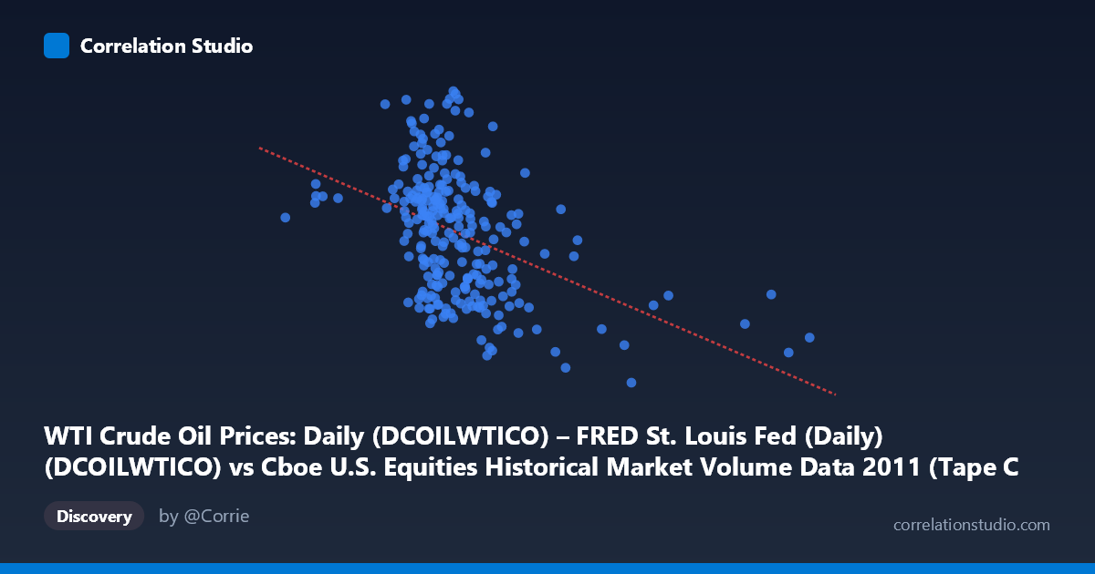
WTI Crude Oil Prices: Daily (DCOILWTICO) – FRED St. Louis Fed (Daily) (DCOILWTICO) vs Cboe U.S. Equities Historical Market Volume Data 2011 (Tape C Trade Count)
- Pearson correlation (r)
- -0.4374
- Spearman correlation
- -0.4402
- p-value
- 0
- Sample size (n)
- 252
- 95% confidence interval
- -0.5322 to -0.3318
- Granger causality
- None
- Granger optimal lag
- 1
AI analysis
Scatterplot Analysis: WTI Crude Oil Prices vs. Cboe Tape C Trade Count (2011)
Relationship Overview
The scatterplot reveals a negative relationship between WTI crude oil prices (x-axis, ranging roughly from $75–$115/barrel) and Cboe Tape C trade counts (y-axis). As oil prices increase, equity trade counts on Tape C tend to decline. The linear regression equation (y = −2.915×10⁻⁵x + 110.85) confirms this downward slope, suggesting that for every $10 increase in WTI prices, Tape C trade counts fall by approximately 0.29 units. However, the scatter around this trend line is considerable, indicating that oil prices alone are far from a complete explanation for trading volume behavior. The relationship is statistically detectable but far from deterministic in nature.
Correlation Strength and Statistical Interpretation
The Pearson correlation of r = −0.437 indicates a moderate negative association. More importantly, the coefficient of determination r² = 0.191 tells us that WTI crude oil prices explain only about 19.1% of the variance in Tape C trade counts — meaning roughly 80.9% of the variation remains unexplained by this single variable. The 95% confidence interval of [−0.532, −0.332] is entirely negative and reasonably tight, suggesting the direction of the relationship is reliable, though the magnitude carries meaningful uncertainty. The p-value of 3.35×10⁻¹³ confirms the correlation is highly statistically significant given the sample size (n = 252 from a population of 3,780), making it extremely unlikely to be a random artifact. That said, statistical significance here is partly a product of the large N and should not be conflated with practical or economic significance. Critically, the Granger causality analysis finds no significant predictive directionality: X→Y yields F = 0.011, p = 0.917 (essentially zero predictive power), and Y→X yields F = 3.477, p = 0.063, which narrowly misses the conventional 0.05 threshold. This means neither variable meaningfully predicts the other's future values, and the observed correlation likely reflects simultaneous co-movement with shared external drivers rather than any causal chain between oil prices and equity trade counts.
Notable Patterns, Clusters, and Outliers
Several features stand out in the sample points. There is a loose central cluster of observations concentrated in the X range of roughly 475,000–600,000 and Y range of 85–105, which likely represents the bulk of typical trading days in 2011. A few notable outliers are visible: the point near (921,203, 85.48) sits far to the right of the main cluster, representing an unusually high oil price day with a relatively low trade count, and could correspond to the oil price spike of spring 2011. Conversely, points like (407,475, 111.68) and (274,733, 101.29) appear at lower oil price levels with higher trade counts. There is also a suggestion of heteroscedasticity — the spread of Y values appears somewhat wider at lower X values, compressing slightly as oil prices rise. No strong non-linear curvature is immediately apparent, but the scatter density does not cleanly conform to a linear pattern, hinting that a segmented or regime-based model might better capture the dynamics.
Confounding Factors and Interpretive Caveats
Several important caveats temper interpretation. 2011 was an unusually volatile year for both oil markets (Arab Spring, Libyan civil war, eurozone debt crisis) and equity markets (U.S. debt ceiling crisis, August 2011 flash crash), meaning both variables were simultaneously driven by macro-risk events that could produce spurious co-movement. Tape C specifically covers NYSE Arca-listed securities (often ETFs and tech stocks), whose trading volumes are sensitive to risk appetite, volatility regimes, and algorithmic trading flows — none of which are directly linked to oil prices. A classic third-variable problem is likely at play: broad market risk sentiment (e.g., VIX), macroeconomic uncertainty, or investor deleveraging episodes could be independently driving both higher oil prices and lower trade counts during stress periods. Additionally, the axes may be swapped in labeling (the dataset descriptions appear transposed in the metadata), which warrants careful verification before drawing firm conclusions.
Actionable Insights and Further Investigation
Despite its limitations, this analysis suggests several productive next steps. First, incorporating the VIX or a broad risk-sentiment index as a control variable would help determine whether the oil–trade count relationship survives after accounting for shared macro-volatility drivers. Second, a regime-segmentation analysis — splitting the data into pre- and post-August 2011 stress periods — could reveal whether the negative correlation is concentrated in specific market episodes rather than being a stable year-round phenomenon. Third, examining other Tape designations (A and B) alongside Tape C would clarify whether this relationship is specific to the exchange segment or broadly systemic. Finally, extending the analysis to multiple years would test whether 2011 is anomalous or representative, and a rolling correlation analysis could reveal whether the r = −0.437 relationship is stable across time or episodic — information that would be essential before using this relationship for any trading or risk management application.
X dataset: Cboe U.S. Equities Historical Market Volume Data 2011
Y dataset: WTI Crude Oil Prices: Daily (DCOILWTICO) – FRED St. Louis Fed (Daily)
Part of experiment: Daily - Cboe U.S. Equities Historical Market Volume Data 2011 vs WTI Crude Oil Prices: Daily (DCOILWTICO) – FRED St. Louis Fed (Daily)