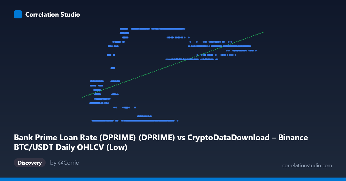
Bank Prime Loan Rate (DPRIME) (DPRIME) vs CryptoDataDownload – Binance BTC/USDT Daily OHLCV (Low)
- Pearson correlation (r)
- 0.4708
- Spearman correlation
- 0.3498
- p-value
- 0
- Sample size (n)
- 2221
- 95% confidence interval
- 0.4378 to 0.5025
- Granger causality
- None
- Granger optimal lag
- 1
AI analysis
Analysis: Bank Prime Loan Rate vs. BTC/USDT Price Data
Note on axis labeling: The metadata appears reversed from what the column names suggest — the X-axis is labeled with the crypto dataset name but described as "Bank Prime Loan Rate," while Y is labeled with the FRED dataset name but described as BTC/USDT Low price. Based on the data ranges (X: 2,817–123,084 resembling BTC price in USD; Y: 3.25–8.50 resembling an interest rate in %), it's most likely that X = BTC/USDT price and Y = Bank Prime Loan Rate. This analysis proceeds on that interpretation.
1. Overview of the Relationship The scatterplot shows a moderate positive association between Bitcoin's price and the U.S. Bank Prime Loan Rate over the 2017–2026 window. As BTC prices rose from the thousands into six-figure territory, the prevailing prime rate also tended to be higher, though the relationship is far from tight or deterministic — there's substantial vertical spread (multiple Y-values) at almost every X-level.
2. Strength, Direction, and Statistical Confidence The correlation coefficient (r = 0.4708) indicates a moderate positive relationship, but r² = 0.2216 means only about 22% of the variance in the prime rate is explained by BTC price (or vice versa) — leaving ~78% attributable to other factors. The 95% CI [0.438, 0.503] is fairly narrow, and the p-value ≈ 0 confirms this correlation is statistically robust and not due to chance, aided by a large sample (n=2,221). However, statistical significance here reflects sample size more than practical strength — this is a weak-to-moderate relationship in real-world terms. Critically, the Granger causality tests show no significant predictive direction (X→Y: p=0.176; Y→X: p=0.439). This means neither variable's past values reliably help forecast the other's future values — the correlation is likely driven by both series trending over the same calendar period (2017–2026) rather than one causing or leading the other.
3. Patterns, Clusters, and Outliers The data shows a stepped/banded pattern rather than a smooth linear cloud, consistent with the prime rate's known behavior of holding constant for extended periods before discrete Fed-driven jumps (e.g., clusters at 3.25%, 5.00%, 6.75%, 7.50%, 8.50%). Within each rate "band," BTC prices vary enormously — e.g., at Y=3.25%, X ranges from ~6,700 to ~62,000, while at Y=8.50%, X ranges from ~34,000 to ~63,000. This banding is the dominant visual feature and explains why linear r² is capped: the relationship is more like a categorical/regime structure than a continuous linear one. No extreme bivariate outliers stand out beyond this natural bandedness.
4. Confounding Factors and Caveats This is a classic spurious/confounded time-series correlation risk: both series are non-stationary and trended upward over overlapping calendar periods (BTC's multi-year bull cycles; Fed's post-2022 hiking cycle). Neither variable causes the other economically in any direct mechanistic sense — the prime rate is set by Fed policy independent of crypto markets, and BTC pricing is driven by market speculation, adoption, and liquidity conditions. The correlation is far more plausibly explained by a shared macro driver (time/monetary policy regime) than genuine interaction. Additionally, mismatched sampling frequency (daily BTC OHLCV vs. FRED's less-frequently-updated prime rate) creates artificial repeated Y-values that inflate apparent banding.
5. Suggested Next Steps - De-trend or difference both series (e.g., BTC log-returns vs. prime rate changes) before testing correlation, to remove the shared-time-trend artifact. - Control for a common third variable, such as broad market liquidity, Fed funds rate expectations, or DXY (dollar index), to test whether the relationship survives. - Given the non-significant Granger results, avoid using one series to forecast the other; instead, treat both as outputs of independent macro regimes rather than a tradable causal pair. - If deeper investigation is warranted, use cointegration testing (e.g., Engle-Granger) rather than simple correlation, since both series are likely trending/non-stationary.
X dataset: CryptoDataDownload – Binance BTC/USDT Daily OHLCV
Y dataset: Bank Prime Loan Rate (DPRIME)
Part of experiment: Bitcoin - CryptoDataDownload – Binance BTC/USDT Daily OHLCV vs Bank Prime Loan Rate (DPRIME)