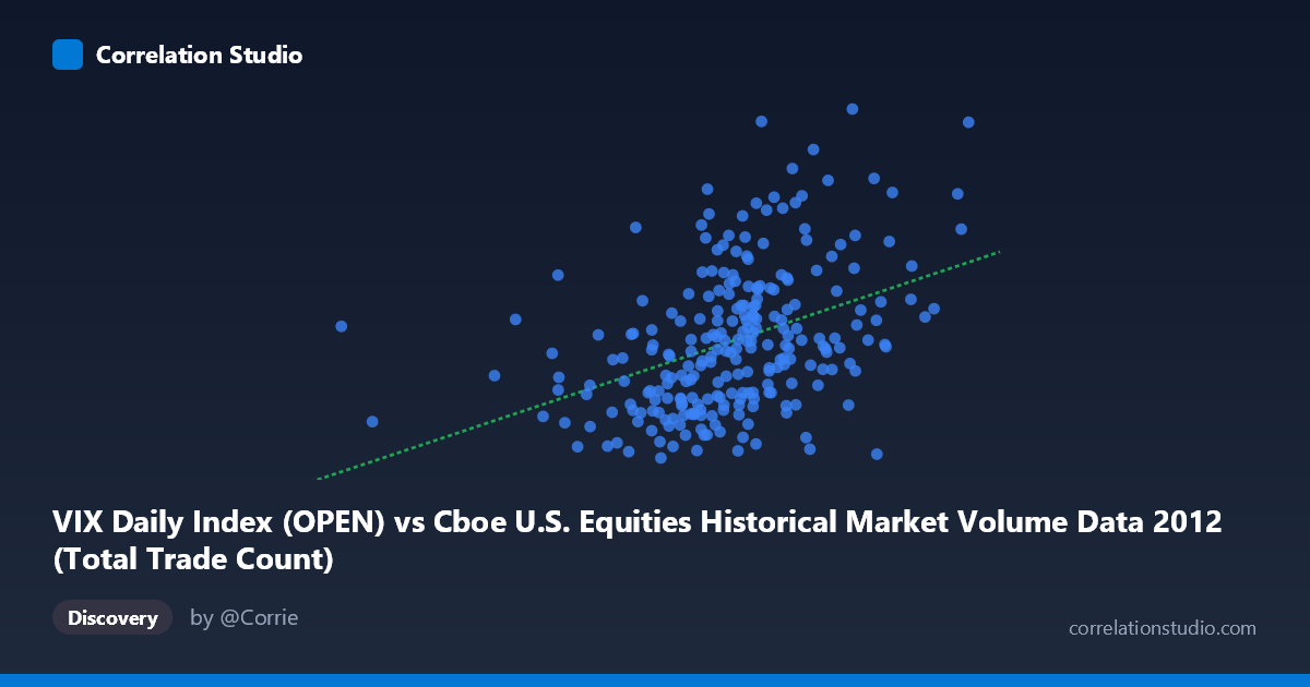
VIX Daily Index (OPEN) vs Cboe U.S. Equities Historical Market Volume Data 2012 (Total Trade Count)
- Pearson correlation (r)
- 0.4093
- Spearman correlation
- 0.4414
- p-value
- 0
- Sample size (n)
- 250
- 95% confidence interval
- 0.3005 to 0.5076
- Granger causality
- None
- Granger optimal lag
- 1
AI analysis
Scatterplot Analysis: VIX Open vs. Total Trade Count (2012)
Relationship Overview The scatterplot reveals a modest positive relationship between the VIX Daily Index (Open) and the Total Trade Count for U.S. equities in 2012. As the VIX — a measure of implied market volatility — rises, total trade counts tend to increase, which aligns intuitively with market behavior: periods of elevated uncertainty typically drive higher trading activity as participants react, hedge, or rebalance positions. However, the relationship is visually noisy, with considerable scatter around the regression line (y = 4.47979E-6x + 10.5527), suggesting that while the trend is real, VIX alone is far from a complete explanation of daily trading volume.
Correlation Strength and Statistical Interpretation The Pearson correlation of r = 0.41 indicates a moderate positive association, but the explanatory power is limited — r² = 0.168 means only ~16.8% of the variance in trade counts is explained by VIX open levels. The remaining ~83% is driven by other factors entirely. The 95% confidence interval [0.30, 0.51] is meaningfully above zero and relatively tight given n = 250, and the p-value of 1.6×10⁻¹¹ confirms the relationship is highly statistically significant — this is not a chance finding. That said, statistical significance should not be conflated with practical significance here; the effect size is moderate at best. Critically, Granger causality tests in both directions are non-significant (X→Y: p = 0.418; Y→X: p = 0.707), meaning neither variable reliably predicts the other in a temporal, lead-lag sense. VIX and trade counts appear to move together contemporaneously rather than one preceding the other, which undermines any causal narrative.
Patterns, Clusters, and Outliers The sample points reveal several notable features. There is a visible cluster of observations in the X range of roughly 1,400,000–1,800,000 with Y values between 15–20, forming the dense core of the dataset. Above Y ≈ 22, points become sparser but are still spread across a wide X range (e.g., points near 1,577,340 with Y = 23.44 and 1,709,830 with Y = 22.93), suggesting high-volatility days don't exclusively correspond to the highest trade counts. Conversely, some low-Y outliers (e.g., Y ≈ 13.68–14.11) occur at moderate X values, indicating that low trade counts can occur even at middling VIX levels. The X-axis spans an unusually wide range (586,356 to 2,284,490), with a few extreme low-volume outliers on the left tail that may disproportionately influence the regression slope.
Confounding Factors and Caveats Several important caveats apply. First, the axes appear swapped in labeling — VIX is plotted on X while trade count is on Y, yet the dataset descriptions suggest the columns may originate from opposite source files, warranting a data provenance check. Second, seasonality is a significant confounder: 2012 trade volumes and VIX both exhibit intra-year patterns (e.g., elevated volatility around the European debt crisis episodes) that could manufacture spurious correlation. Third, day-of-week effects, options expiration cycles, and macro announcements independently drive both variables. Fourth, the population of N = 3,750 versus the sample of n = 250 means the sample represents only ~6.7% of the population — if the sampling is not random across all market regimes, estimates may be biased.
Actionable Insights and Further Investigation Given the moderate correlation without Granger-causal support, practitioners should avoid using VIX as a standalone predictor of trade volume. Recommended next steps include: (1) decomposing the analysis by volatility regime (low/medium/high VIX terciles) to test whether the relationship strengthens nonlinearly above a VIX threshold (e.g., VIX 20); (2) incorporating additional predictors such as S&P 500 returns, bid-ask spreads, or news sentiment to build a multivariate model that captures the missing ~83% of variance; (3) testing for lagged relationships at longer horizons (2–5 days) since the optimal lag of 1 period showed no significance; and (4) applying a time-series decomposition to remove shared seasonal trends before re-examining the correlation, ensuring the observed relationship reflects genuine co-movement rather than shared temporal structure.
X dataset: Cboe U.S. Equities Historical Market Volume Data 2012
Y dataset: VIX Daily Index
Part of experiment: Daily - Cboe U.S. Equities Historical Market Volume Data 2012 vs VIX Daily Index