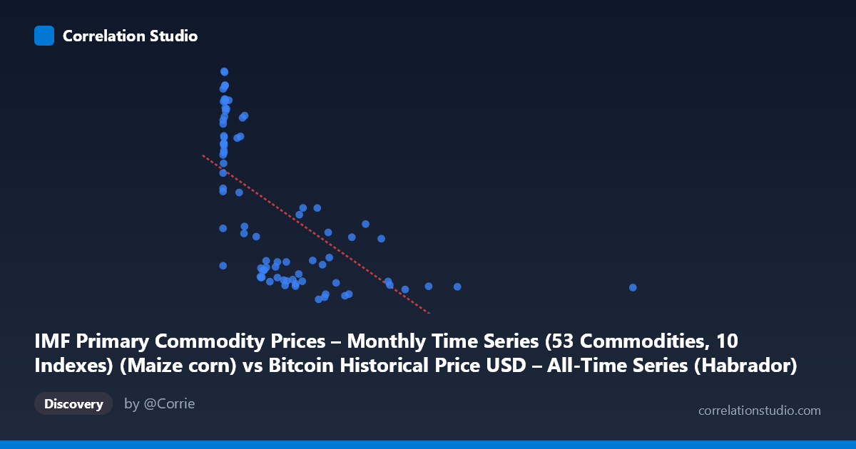
IMF Primary Commodity Prices – Monthly Time Series (53 Commodities, 10 Indexes) (Maize corn) vs Bitcoin Historical Price USD – All-Time Series (Habrador) (Price)
- Pearson correlation (r)
- -0.6323
- Spearman correlation
- -0.7271
- p-value
- 0
- Sample size (n)
- 83
- 95% confidence interval
- -0.7462 to -0.4824
- Granger causality
- None
- Granger optimal lag
- 10
- Time coverage
- 2010-08-01 to 2017-06-01
- Recomputed on refreshed data
- 2026-10-24 (r was -0.6323)
AI analysis
Analysis: Bitcoin Price vs. Maize Corn Index
1. What the Scatterplot Reveals
The visualization shows a clear negative, non-linear relationship between the two variables. At low X-axis values (roughly 0–200), Y values are widely scattered across a high range (~200–333), forming a dense vertical cluster near the origin. As X increases beyond ~200, Y values drop sharply and then flatten into a tight, low band (~150–165) that persists even as X extends out to 2452. This pattern resembles a decaying exponential or power-law relationship rather than a straight line, with most of the "action" concentrated in the low-X region.
2. Strength, Direction, and Statistical Confidence
The Pearson correlation of r = -0.632 indicates a moderate-to-strong negative linear association, with r² = 0.40 meaning that a linear model explains only 40% of the variance in Y — leaving the majority (60%) unexplained by X alone. This is consistent with the visibly curved, non-linear shape of the data, which a linear model tends to underfit. The 95% CI [-0.746, -0.482] is reasonably narrow and does not cross zero, and the p-value (1.44E-10) is highly significant, so we can be confident a real negative relationship exists — but confidence in the linear correlation coefficient doesn't validate linearity itself. Critically, the Granger causality tests show no significant predictive direction in either direction (X→Y p=0.294; Y→X p=0.119). This means that despite the strong contemporaneous correlation, neither variable's past values reliably help forecast the other's future values at the tested lag structure — undermining any causal or leading-indicator interpretation.
3. Notable Patterns and Outliers
- Two-regime structure: A high-Y/low-X cluster (X < 200, Y 200) and a low-Y/high-X cluster (X 200, Y < 220) suggest the relationship may be better modeled as a threshold, log, or inverse function rather than linear. - Extreme X outlier: The point (2452.18, 157.96) sits far beyond the rest of the data (next highest X ~1402), heavily influencing the linear slope and r value despite being a single observation. - Y-axis spread at low X: Points like (6.63, 332.95) and (0.06, 205.84) show huge Y variability when X is near zero, indicating X has little explanatory power in that region — the negative correlation is driven largely by the high-X tail. - Compression at high X: Once X exceeds ~600, Y values converge tightly to 150–220, suggesting diminishing sensitivity (saturation effect).
4. Confounding Factors and Caveats
Both series are monthly time series spanning 2010–2017, meaning autocorrelation and shared macro trends (not necessarily causal linkage between Bitcoin and corn prices) could be driving the correlation. Bitcoin's price is dominated by exponential speculative growth phases, while commodity indexes respond to agricultural/economic cycles — any apparent relationship may be spurious, reflecting two unrelated series that happen to have inversely-timed trends over this specific window (e.g., corn prices declining post-2012 while Bitcoin remained low, then Bitcoin's 2017 explosive rally). The lack of Granger causality reinforces that this is likely a coincidental trend alignment rather than a mechanistic relationship. Additionally, the sample (n=83) is much smaller than the reported population (N=449), so results may not generalize to the full time series.
5. Actionable Insights
- Avoid linear modeling: Given the curvature, log-transforming X (or Y) or fitting a power/exponential decay model would likely substantially improve fit over the current r²=0.40. - Investigate the extreme outlier: Re-run correlation/regression excluding the (2452.18, 157.96) point to test robustness of the reported r. - Treat as spurious/confounded until proven otherwise: Given no Granger causality, this correlation should not be used for trading signals or forecasting one series from the other. Any narrative connecting Bitcoin prices to corn/commodity prices needs a plausible economic mechanism (e.g., shared macro liquidity, inflation, USD strength) tested directly rather than inferred from this bivariate correlation alone. - Segment by time regime: Given Bitcoin's known regime shifts (2011 bubble, 2013 bubble, 2017 bubble), consider splitting the analysis by sub-periods to see if the relationship is stable or an artifact of one particular era.
X dataset: Bitcoin Historical Price USD – All-Time Series (Habrador)
Y dataset: IMF Primary Commodity Prices – Monthly Time Series (53 Commodities, 10 Indexes)
Part of experiment: Bitcoin - Bitcoin Historical Price USD – All-Time Series (Habrador) vs IMF Primary Commodity Prices – Monthly Time Series (53 Commodities, 10 Indexes)