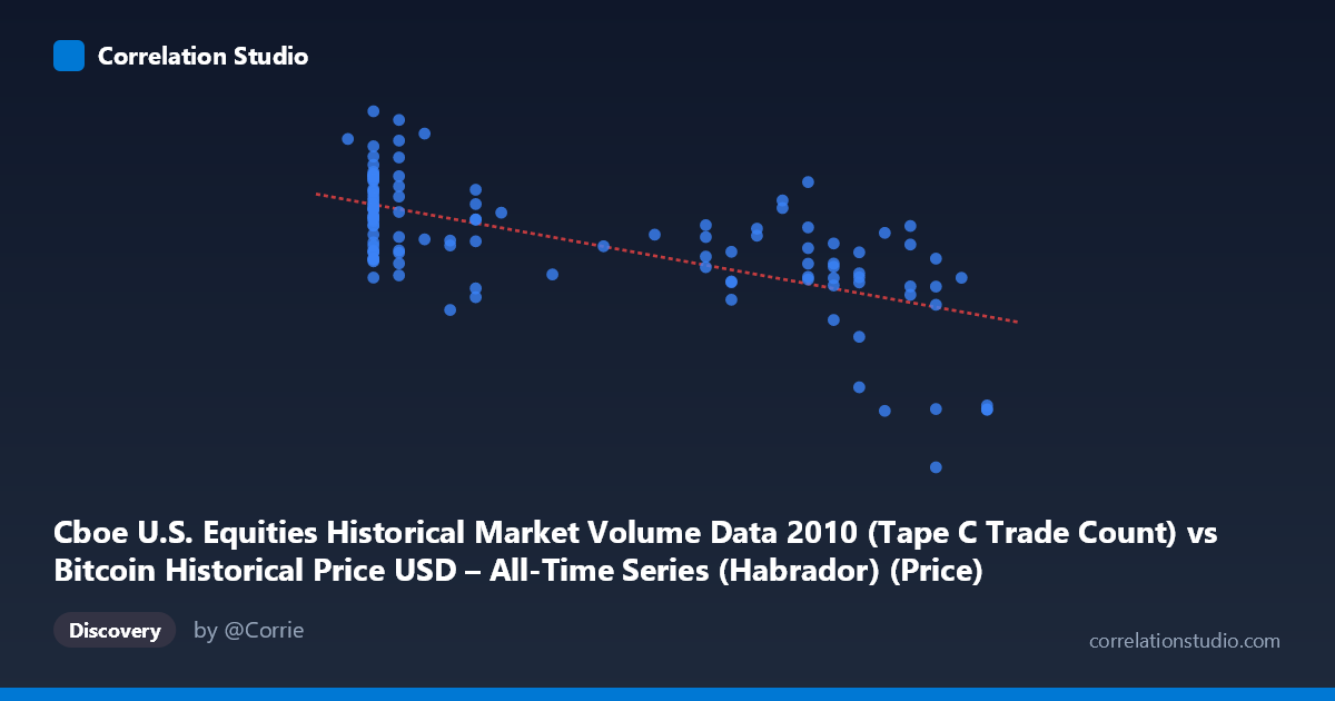
Cboe U.S. Equities Historical Market Volume Data 2010 (Tape C Trade Count) vs Bitcoin Historical Price USD – All-Time Series (Habrador) (Price)
- Pearson correlation (r)
- -0.6537
- Spearman correlation
- -0.6346
- p-value
- 0
- Sample size (n)
- 117
- 95% confidence interval
- -0.7466 to -0.5357
- Granger causality
- None
- Granger optimal lag
- 10
- Time coverage
- 2010-07-19 to 2010-12-31
AI analysis
Analysis of the Relationship Between Trade Count and Bitcoin Price
1. What the Visualization Reveals
The scatterplot shows a moderate negative linear relationship between the Cboe Tape C trade count and Bitcoin's daily USD price during the latter half of 2010. As trade counts increase from roughly 0.06 to 0.30 (in normalized/scaled units), Bitcoin prices tend to decline from a cluster of high values (~500,000–730,000) down to a distinct low cluster (~260,000–270,000) at the highest trade count values. The regression line (y = -727,480x + 627,062) captures this downward trend, though there is considerable scatter around it, especially in the low-to-mid X range.
2. Strength, Direction, and Statistical Confidence
The correlation coefficient of r = -0.6537 indicates a moderately strong negative relationship, with r² = 0.4273 meaning that only about 43% of the variance in Bitcoin price is explained by trade count — leaving the majority (57%) attributable to other factors or noise. The 95% confidence interval [-0.7466, -0.5357] is reasonably tight and entirely negative, and the p-value (1.33e-15) confirms this correlation is highly statistically significant and not due to chance in this sample. However, the Granger causality tests (F = 0.84, p = 0.59 for X→Y; F = 0.88, p = 0.56 for Y→X) show no significant predictive temporal relationship in either direction. This is a critical distinction: the variables are statistically associated in a cross-sectional/contemporaneous sense, but neither reliably precedes or forecasts the other over time at the tested lag structure.
3. Notable Patterns and Clusters
The data reveals distinct clustering rather than a smooth continuous trend. A dense cluster sits at low X (~0.06–0.11) with high, variable Y values (438,000–729,000) — this cluster alone shows substantial vertical spread, suggesting X is a weak predictor within this region. A second, tighter cluster appears at high X (~0.19–0.28) with more moderate Y values (400,000–590,000). A distinct outlier group at X ≈ 0.30 shows sharply lower Y values (~263,000–270,000), which appears to be pulling the regression slope and correlation strength considerably — these few points may be exerting outsized leverage. Without them, the relationship would likely appear weaker.
4. Confounding Factors and Caveats
Both time series span the same period (mid-to-late 2010), so any shared trend — such as both variables reacting to overall market growth, seasonality, or external events — could produce a spurious correlation without genuine causal linkage. Since Bitcoin traded at minuscule volumes and prices in 2010, and Tape C trade counts reflect broad U.S. equity market activity, there is no obvious economic mechanism directly connecting them; the correlation may be an artifact of both being monotonic/trending time series (a classic spurious-correlation scenario in time series analysis). The lack of Granger causality reinforces suspicion that this is correlation without demonstrable directional influence. Additionally, the small n (117) sampled from a larger population (3,302) means clustering artifacts or sampling choices could distort the apparent linear fit.
5. Suggestions for Further Investigation
Given the spurious-correlation risk with two unrelated trending time series, analysts should test for cointegration or difference/detrend both series before assessing correlation, and rerun Granger tests on stationary (differenced) data rather than levels. It would also be valuable to examine whether both series are simply increasing/decreasing over the sample period due to independent trends (Bitcoin's 2010 price rally/correction vs. equity market volume patterns), which could fully explain the r² without implying any real-world interaction. Finally, isolating and investigating the high-X outlier cluster (X ≈ 0.30) separately would clarify whether the overall correlation is being driven by a handful of extreme observations rather than a genuine relationship across the full range.
X dataset: Bitcoin Historical Price USD – All-Time Series (Habrador)
Y dataset: Cboe U.S. Equities Historical Market Volume Data 2010
Part of experiment: Bitcoin - Bitcoin Historical Price USD – All-Time Series (Habrador) vs Cboe U.S. Equities Historical Market Volume Data 2010