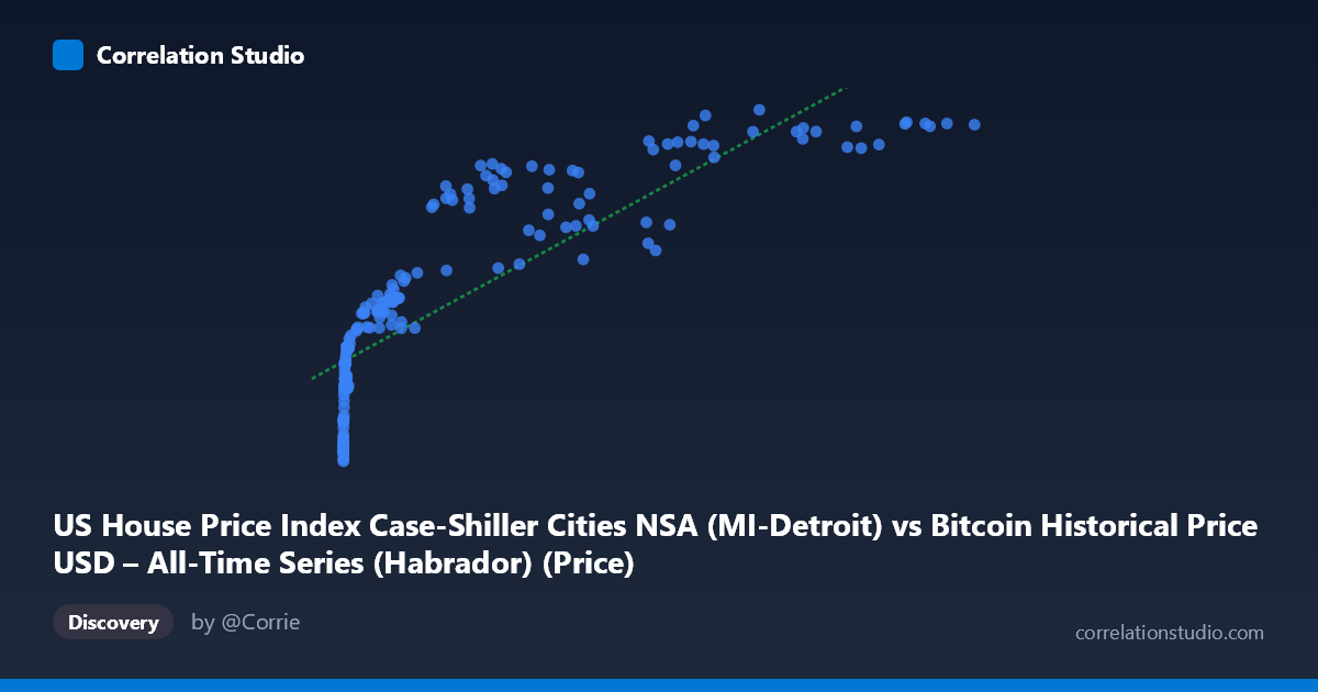
US House Price Index Case-Shiller Cities NSA (MI-Detroit) vs Bitcoin Historical Price USD – All-Time Series (Habrador) (Price)
- Pearson correlation (r)
- 0.835
- Spearman correlation
- 0.972
- p-value
- 0
- Sample size (n)
- 186
- 95% confidence interval
- 0.7855 to 0.8739
- Granger causality
- None
- Granger optimal lag
- 1
AI analysis
Analysis: Bitcoin Price vs. Detroit Case-Shiller Home Price Index
1. What the Visualization Reveals
The scatterplot shows a strong, positive, but clearly non-linear relationship between Bitcoin's USD price and the Detroit metro home price index. At low Bitcoin values (under ~$1,000), the Case-Shiller index clusters tightly between roughly 65-115, showing steep relative movement in Y for tiny changes in X. As Bitcoin climbs into the tens of thousands, the home price index rises more gradually and begins to plateau near 180-199. This is the classic signature of a logarithmic curve: Y increases rapidly with X at low values and flattens as X grows large — consistent with the note that Spearman's ρ exceeds Pearson's r.
2. Strength, Direction, and Uncertainty
The linear Pearson correlation (r = 0.835, R² = 0.697) indicates a strong positive association, with roughly 70% of variance in Y "explained" by X in a linear model. The 95% CI [0.786, 0.874] is tight and the p-value is effectively zero, so the correlation is statistically robust and not a product of sampling noise — but statistical significance here reflects the shared upward trend over time, not necessarily a meaningful causal or economic link. Critically, the Granger causality tests show no significant predictive direction in either direction (X→Y: p=0.322; Y→X: p=0.0996, only marginally suggestive). This strongly implies that neither series temporally leads the other — they are likely both driven by a common underlying factor (time itself, or macroeconomic conditions like inflation, monetary expansion, and risk appetite) rather than one causing the other.
3. Notable Patterns and Outliers
Several features stand out: - Two-regime clustering: a dense cloud of points at very low X (Bitcoin < $1,000, pre-2017) with Y between 65-125, and a sparser, more scattered cloud at high X (Bitcoin $20,000) with Y between 140-199. - Compression at high X: multiple Bitcoin prices between $85,000-$118,000 all map to a narrow Y band (~195-199), indicating index saturation — home prices stop responding to further Bitcoin appreciation. - Vertical scatter at similar X: e.g., near X≈57,000-62,000, Y ranges from 148 to 191 — showing that at a given Bitcoin price level, the home index value varies considerably depending on when that price occurred (time-lag effects), reinforcing that this is largely a time-trend artifact. - No obvious reversals or negative excursions — the relationship is monotonic overall.
4. Confounders and Caveats
This correlation is almost certainly spurious or trend-driven rather than causal: - Shared time trend: Both Bitcoin price and home price indices have risen dramatically since 2010-2026, driven by unrelated but overlapping macro forces (loose monetary policy, low interest rates, inflation, speculative demand). Two unrelated upward-trending series will often correlate strongly. - Non-stationarity: Neither series is mean-reverting; both have long-term secular growth, which inflates correlation coefficients and undermines the validity of Granger causality tests (which assume stationarity) — the marginal Y→X result (p=0.0996) should be treated cautiously. - Scale mismatch: X spans 6 orders of magnitude while Y spans about 3-fold — the regression is highly sensitive to the extreme high-X points (Bitcoin's later bull runs). - No plausible economic mechanism directly links Bitcoin price to Detroit-specific housing costs.
5. Actionable Insights
- Refit with a log transform: Given the shape, model Y ~ log(X) rather than a linear fit; this should substantially improve fit quality and better reflect the diminishing-returns relationship visible in the scatter. - Detrend before testing causality: Apply differencing or growth-rate transformations to both series (e.g., % change month-over-month) and re-run correlation/Granger tests on stationary series to see if any genuine short-term relationship survives once the common trend is removed. - Treat this as a trend-correlation, not a trading/economic signal: Given the lack of Granger causality, this pairing is unsuitable for predictive modeling (e.g., using Bitcoin to forecast Detroit home prices or vice versa). - Investigate common drivers directly: A more informative analysis would examine both series against shared macro variables (M2 money supply, federal funds rate, inflation/CPI) to identify the true common cause of their parallel trends.
X dataset: Bitcoin Historical Price USD – All-Time Series (Habrador)
Y dataset: US House Price Index Case-Shiller Cities NSA
Part of experiment: Bitcoin - Bitcoin Historical Price USD – All-Time Series (Habrador) vs US House Price Index Case-Shiller Cities NSA