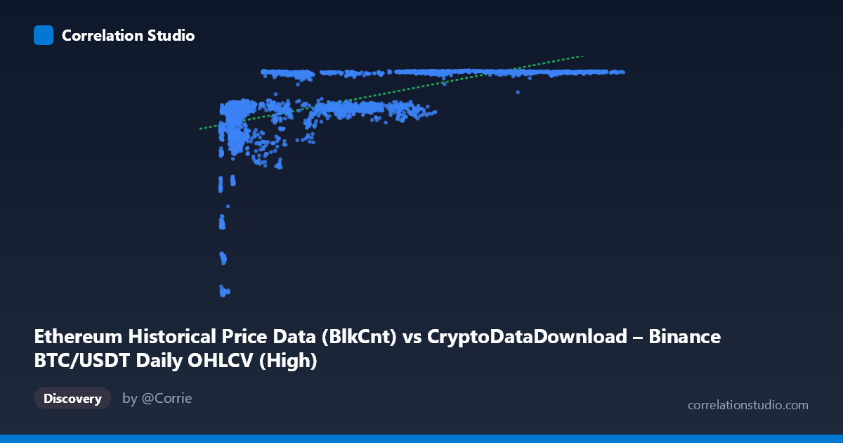
Ethereum Historical Price Data (BlkCnt) vs CryptoDataDownload – Binance BTC/USDT Daily OHLCV (High)
- Pearson correlation (r)
- 0.5719
- Spearman correlation
- 0.7283
- p-value
- 0
- Sample size (n)
- 3191
- 95% confidence interval
- 0.5481 to 0.5948
- Granger causality
- None
- Granger optimal lag
- 1
AI analysis
Analysis of BTC/ETH-Related Metric Correlation
1. What the Visualization Reveals
The scatterplot shows a positive but non-linear relationship between the X variable (labeled as block count, though the range and description suggest it may actually be a price or volume-related metric) and Y (BTC/USDT daily high price). The pattern is not a clean linear cloud — it strongly resembles a logarithmic or saturating curve: Y rises steeply as X increases from its minimum (~3,300) up to roughly 20,000–30,000, then flattens into a plateau around 7,100–7,180 for the remainder of the X range (up to 126,000). This "rapid rise then plateau" shape is the dominant visual feature.
2. Strength, Direction, and Statistical Confidence
The Pearson correlation (r = 0.572) indicates a moderate positive linear association, with r² = 0.327 meaning the linear model explains only ~33% of the variance in Y — leaving two-thirds unexplained by a straight-line fit. The 95% CI [0.548, 0.595] is tight and the p-value is effectively 0, so we can be confident a linear relationship exists and is not due to chance — but statistical significance here reflects the large sample size (n=3,191), not necessarily practical strength or correct functional form. The note that Spearman's ρ exceeds Pearson's r confirms the visual impression: a monotonic but curved (logarithmic-type) relationship fits better than a straight line, meaning the true explanatory power is likely higher than 32.7% once non-linearity is modeled. Critically, the Granger causality tests show no significant predictive direction in either direction (X→Y p=0.51, Y→X p=0.82), indicating that despite the contemporaneous correlation, neither series helps forecast the other's future values at lag 1 — this is consistent with both being driven by a common external factor (likely overall market conditions/time trend) rather than one causing the other.
3. Notable Patterns and Outliers
- Low-X cluster (X < 10,000): Y values are highly dispersed (2,829–6,500), including the dataset's lowest Y points (e.g., 4,380→2,840; 4,367→3,499; 3,873→4,238). This is the noisiest region and likely corresponds to an early/bear-market period. - Plateau region (X 25,000): Y compresses tightly into a narrow band (~6,300–7,180), suggesting a price ceiling or resistance level reached during a bull run, with diminishing sensitivity to X. - Vertical banding: Multiple X values map to nearly identical Y (e.g., ~7,140–7,178 recurring across X = 28,000 to 111,000), reinforcing the saturation effect rather than continued linear growth. - No dramatic negative outliers are apparent; the "outlier" behavior is concentrated in the low-X tail where variance is highest.
4. Confounding Factors and Caveats
- Time is a likely confound: Both series span 2017–2026, covering multiple BTC/ETH market cycles. Trends over time (bull/bear cycles) can induce spurious correlation between two unrelated series that both drift upward over the period. - Metric mismatch/labeling ambiguity: The X-axis label ("BlkCnt") and description (price OHLCV) are inconsistent, raising concern about data alignment or mislabeling — this should be verified before drawing conclusions. - Autocorrelation: Daily financial/network data is highly autocorrelated, which can inflate apparent correlation and distort Granger test assumptions (lag=1 may be insufficient). - Non-stationarity: Crypto price/volume data is typically non-stationary; failing to difference or detrend before correlation/Granger analysis can produce misleading results.
5. Suggested Next Steps
1. Fit a logarithmic or power model (e.g., Y ~ log(X)) and compare R² against the linear 32.7% — likely to show meaningfully better fit given the Spearman/Pearson gap. 2. Detrend or difference both series (e.g., use daily returns/changes rather than levels) and re-run correlation and Granger tests to rule out shared time-trend confounding. 3. Clarify data provenance — confirm whether X truly represents block count, price, or another metric, given the labeling inconsistency. 4. Segment analysis by market regime (bull vs. bear periods) to see if the relationship strength/shape differs across cycles. 5. Test longer Granger lags (e.g., 5, 10, 30 days) since crypto market effects often propagate over multiple days/weeks, not just one lag period.
X dataset: CryptoDataDownload – Binance BTC/USDT Daily OHLCV
Y dataset: Ethereum Historical Price Data
Part of experiment: Bitcoin - CryptoDataDownload – Binance BTC/USDT Daily OHLCV vs Ethereum Historical Price Data