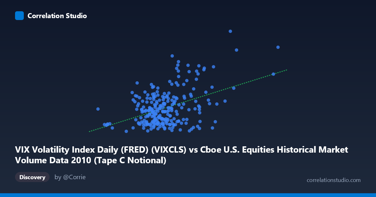
VIX Volatility Index Daily (FRED) (VIXCLS) vs Cboe U.S. Equities Historical Market Volume Data 2010 (Tape C Notional)
- Pearson correlation (r)
- 0.4363
- Spearman correlation
- 0.2604
- p-value
- 0
- Sample size (n)
- 252
- 95% confidence interval
- 0.3306 to 0.5313
- Granger causality
- Y → X
- Granger optimal lag
- 1
AI analysis
VIX Volatility Index vs. Cboe Tape C Notional Volume (2010)
Relationship Overview The scatterplot reveals a positive relationship between Cboe Tape C notional trading volume (X-axis) and the VIX Volatility Index (Y-axis) across 252 trading days in 2010. The linear regression equation (y = 2.35×10⁻⁹x + 13.32) confirms that as notional volume increases, VIX levels tend to rise — a directionally intuitive finding, since market stress and fear (captured by VIX) typically coincide with elevated trading activity as participants rush to hedge or liquidate positions. However, the relationship is visually diffuse, with considerable vertical scatter at any given volume level, signaling that volume alone is far from a complete predictor of volatility.
Correlation Strength and Statistical Significance The Pearson correlation of r = 0.44 indicates a moderate positive association, but the more telling figure is r² = 0.19, meaning notional volume explains only about 19% of the variance in VIX — the remaining 81% is driven by factors not captured here. The 95% confidence interval of [0.33, 0.53] is reasonably tight and does not include zero, and the p-value of 3.89×10⁻¹³ confirms the result is highly statistically significant given n = 252 paired observations drawn from a population of N = 3,302. Critically, Granger causality runs unidirectionally from VIX → Notional Volume (F = 7.10, p = 0.008), not the reverse (F = 1.90, p = 0.169). This means past VIX readings have meaningful temporal predictive power over subsequent trading volume, but past volume does not reliably predict future VIX — an important asymmetry that reframes the causal narrative.
Notable Patterns, Clusters, and Outliers Several structural features stand out in the data: - A dense core cluster sits between roughly 2.5–5.0 billion in notional volume and VIX levels of 15–25, representing typical low-to-moderate volatility trading days that dominated much of 2010's relatively calm post-crisis environment. - A high-volume, high-VIX tail is visible at the upper right, including the notable outlier at approximately (8.48B, 40.95) — almost certainly tied to the May 6, 2010 Flash Crash, when VIX spiked and volume surged dramatically. - Additional elevated-VIX points (35–46 range) at moderate-to-high volumes (5–7B) likely correspond to the European sovereign debt crisis episodes (Greek/Spanish contagion fears) that episodically spiked volatility in mid-2010. - A separate low-VIX cluster (15–18) spans a wide range of volumes (~2–6B), suggesting that low volatility periods are consistent regardless of volume, weakening the linear model's fit across the full range.
Confounding Factors and Caveats Several important caveats apply. First, 2010 was a structurally unusual year — sandwiched between the 2008–09 financial crisis aftermath and the emergence of post-crisis algorithmic and high-frequency trading dominance — making volume dynamics potentially non-stationary. Second, Tape C notional volume represents only a subset of U.S. equity trading (NYSE Arca-listed securities), not total market volume, so it is an incomplete proxy for aggregate market activity. Third, VIX is forward-looking (30-day implied volatility), while notional volume is a contemporaneous realized measure — comparing them introduces an inherent temporal mismatch. Fourth, lurking variables such as Federal Reserve policy announcements, macroeconomic data releases, and index rebalancing events likely co-drive both series simultaneously, inflating the observed correlation through common causation rather than direct linkage.
Actionable Insights and Further Investigation The Granger causality finding — that VIX leads volume rather than the reverse — is the most operationally useful result here. Traders and risk managers could use elevated VIX readings as an early signal of impending volume surges, with a 1-period (1-day) lag, which has practical implications for liquidity planning and execution strategy. To deepen this analysis, investigators should: (1) stratify the data by market regime (e.g., pre/post Flash Crash) to test whether the relationship is structurally stable; (2) include total cross-exchange notional volume rather than Tape C alone; (3) test non-linear models (e.g., log-log or piecewise regression), given the apparent curvilinear behavior at high VIX/volume extremes; and (4) extend the time series beyond 2010 to assess whether the VIX→Volume Granger relationship persists across different volatility regimes and market microstructure conditions.
X dataset: Cboe U.S. Equities Historical Market Volume Data 2010
Y dataset: VIX Volatility Index Daily (FRED)
Part of experiment: Daily - Cboe U.S. Equities Historical Market Volume Data 2010 vs VIX Volatility Index Daily (FRED)