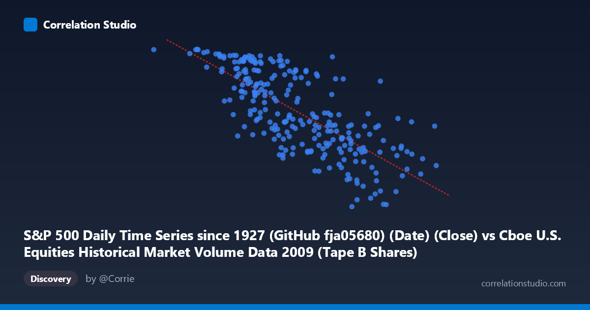
S&P 500 Daily Time Series since 1927 (GitHub fja05680) (Date) (Close) vs Cboe U.S. Equities Historical Market Volume Data 2009 (Tape B Shares)

Pearson correlation (r): -0.7453
Spearman correlation: -0.7582
p-value: 0
Sample size (n): 252
95% confidence interval: -0.7956 to -0.6848
Granger causality: Bidirectional
Granger optimal lag: 10

AI analysis

Scatterplot Analysis: S&P 500 Close Price vs. Cboe Tape B Share Volume (2009)

Relationship Overview

The scatterplot reveals a moderately strong negative relationship between the S&P 500 closing price (X-axis) and Cboe Tape B share volume (Y-axis) across 252 trading days in 2009. As the S&P 500 index level increases — moving from the crisis lows of early 2009 (~33.8M range low) toward the year-end recovery (~255.8M range high) — Tape B share volume tends to decline systematically. The linear regression equation (y = -2.01356E-06x + 1243.72) makes this concrete: for every unit increase in the S&P 500 close, Tape B volume decreases by approximately 0.000002 units, reflecting a broad secular trend where panic-driven high-volume trading subsided as markets recovered throughout 2009.

Correlation Strength and Statistical Significance

The Pearson correlation of r = -0.7453 indicates a strong negative association, and the r² of 0.5555 means that approximately 55.5% of the variance in Tape B share volume is explained by the S&P 500 price level — a substantial but not complete relationship, leaving roughly 44.5% attributable to other factors. The 95% confidence interval of [-0.7956, -0.6848] is relatively tight and does not approach zero, reinforcing confidence in the direction and magnitude of this effect. The p-value of essentially 0 across a paired sample of n=252 drawn from a population of N=3,232 confirms this is not a chance finding. Critically, the bidirectional Granger causality result (X→Y: F=2.45, p=0.0086; Y→X: F=2.79, p=0.0028) at an optimal lag of 10 trading periods suggests that neither variable is purely the driver — past S&P 500 levels help predict future Tape B volume and past Tape B volume helps predict future S&P 500 levels. This bidirectionality complicates simple causal narratives and points toward a reflexive feedback loop rather than a clean directional cause-and-effect relationship.

Notable Patterns, Clusters, and Outliers

Several structural features stand out in the data distribution. There is a visible cluster of high-volume, low-price observations at the left end of the X-axis (index levels below ~100M), corresponding to the market distress period of early 2009 — the post-financial-crisis panic phase when both volatility and trading activity were elevated. Conversely, a cluster of lower-volume, higher-price points occupies the right side, reflecting the calmer, recovering market of mid-to-late 2009. A few notable outliers are apparent: the point near (33,822,027, 1126.48) shows an exceptionally low X value paired with high Y volume, likely representing the depths of the bear market; and points around (254,504,132, 907.39) and (225,663,058, 929.23) show high X values with unexpectedly elevated volume relative to the trend, possibly reflecting specific high-activity events late in the year. The scatter also widens at lower price levels, suggesting heteroscedasticity — volume becomes more variable and harder to predict during market stress periods.

Confounding Factors and Interpretive Caveats

Several important caveats temper a straightforward causal interpretation. Most fundamentally, both variables are time-indexed to 2009, meaning that the apparent correlation may largely be a spurious artifact of shared temporal trends — both variables are co-evolving through the same macro crisis-to-recovery arc rather than one mechanistically causing the other. The bidirectional Granger result reinforces that the relationship is entangled with time dynamics. Additionally, Tape B specifically covers NYSE MKT (AMEX) and regional exchange securities, which may not uniformly track S&P 500 large-cap movements, introducing systematic noise. Market microstructure changes in 2009, including the rise of high-frequency trading, regulatory shifts post-crisis, and changing retail participation, could independently influence Tape B volumes. The dataset's X-axis label appears to encode dates as numerical values rather than actual index prices — if X represents date ordinals rather than close prices, the entire interpretation shifts toward a time-trend regression rather than a price-volume relationship, which would be a critical reframing.

Actionable Insights and Further Investigation

Practitioners and researchers should pursue several follow-up analyses. First, decomposing the time series using detrending or first-differencing would help isolate whether the correlation persists after removing the shared 2009 recovery trend, which would clarify whether this is a genuine price-volume relationship or a spurious temporal artifact. Second, given the bidirectional Granger causality at a 10-day lag, a trading signal backtest exploring whether Tape B volume spikes at t predict S&P 500 moves at t+10 (and vice versa) could have practical value for short-term market timing. Third, extending the analysis across multiple years (pre-crisis 2006–2007, crisis 2008, recovery 2010–2011) would reveal whether the negative correlation is specific to the crisis-recovery dynamic or a persistent structural relationship. Finally, segmenting the data by VIX regime (high/low volatility periods) would test whether the heteroscedasticity observed in the scatter is driven by volatility clustering, which has direct implications for risk modeling in fragmented equity market structures.

X dataset: Cboe U.S. Equities Historical Market Volume Data 2009

Y dataset: S&P 500 Daily Time Series since 1927 (GitHub fja05680) (Date)

Part of experiment: Daily - Cboe U.S. Equities Historical Market Volume Data 2009 vs S&P 500 Daily Time Series since 1927 (GitHub fja05680) (Date)