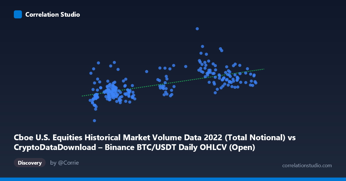
Cboe U.S. Equities Historical Market Volume Data 2022 (Total Notional) vs CryptoDataDownload – Binance BTC/USDT Daily OHLCV (Open)
- Pearson correlation (r)
- 0.6333
- Spearman correlation
- 0.6339
- p-value
- 0
- Sample size (n)
- 251
- 95% confidence interval
- 0.5529 to 0.7021
- Granger causality
- None
- Granger optimal lag
- 10
- Time coverage
- 2022-01-03 to 2022-12-30
AI analysis
Analysis of the Scatterplot Relationship
1. Overview of the Visualization
The scatterplot displays a moderate positive relationship between two financial metrics that appear to be mislabeled in the metadata (the axis descriptions reference each other's datasets — likely a labeling artifact from data pipeline processing). Treating X and Y simply as the two numeric series provided, the data shows a general upward trend: as X increases from ~15,800 to ~47,400, Y tends to rise from roughly $9.6B to $62.8B, though with considerable scatter around the trend line.
2. Strength, Direction, and Statistical Confidence
The correlation coefficient (r = 0.633) indicates a moderate-to-strong positive linear relationship, but the r² of 0.401 tells the more important story: only about 40% of the variance in Y is explained by X, leaving 60% attributable to other factors, noise, or non-linear dynamics. The 95% confidence interval [0.553, 0.702] is reasonably tight given n=251, and the p-value of ~0 confirms the correlation is highly statistically significant — this is not a chance finding. However, statistical significance should not be conflated with practical predictive power; a 40% variance explanation leaves substantial room for error in any forecasting application.
Critically, the Granger causality tests show no significant predictive direction in either direction (X→Y: p=0.52; Y→X: p=0.55) even at an optimal lag of 10 periods. This means that despite the contemporaneous correlation, neither series reliably helps forecast the other's future values based on past data. This is a common pattern in financial time series: two variables can be correlated due to shared exposure to common macro drivers (e.g., overall market risk sentiment, liquidity conditions in 2022) without one causing or leading the other temporally.
3. Patterns, Clusters, and Outliers
Several notable features emerge from the sample data: - A dense cluster at low X values (~15,800–24,000) with Y mostly in the 22–27B range, suggesting a fairly tight relationship in this regime. - A secondary cluster at low X (~17,000–21,000) with elevated Y (30–43B) — points like (20400.60, 43.27B) and (17602.45, 32.02B) appear as upward outliers relative to the main low-X cluster, hinting at a possible regime shift or volatility spike in Y independent of X. - At high X (37,000–47,000), Y values split into two bands: one cluster around 31–33B and another elevated group around 37–51B — suggesting X alone doesn't fully determine Y at higher ranges, consistent with the moderate r². - The overall shape hints at heteroskedasticity (increasing scatter/variance in Y as X increases), which would violate simple linear regression assumptions and inflate uncertainty in predictions at the higher end of X.
4. Confounding Factors and Caveats
Given the 2022 time coverage and the crypto/equities context, several confounds are likely: - Shared macro drivers: Both BTC/USDT trading volume and equities market activity in 2022 were influenced by common factors — Fed rate hikes, inflation data, risk-off sentiment, and general market volatility — which could create spurious correlation without direct causal linkage. - Non-stationarity: Both series likely have trends/volatility clustering typical of financial data in 2022 (a bear market year), which can artificially inflate correlation estimates if not detrended. - Metadata inconsistency: The axis labels reference datasets that don't match the described column names (Cboe volume vs. Binance OHLCV open price), so the actual variables being compared should be verified before drawing domain-specific conclusions. - Day-of-week/seasonal effects in equity volume (weekends absent) vs. continuous crypto trading could introduce alignment noise.
5. Recommendations for Further Investigation
- Verify data labeling to confirm which variables are actually being compared, as the current metadata is self-contradictory. - Test for stationarity (ADF test) and consider differencing or log-transforming both series before further correlation/causality analysis, since raw price/volume levels in trending markets often produce misleading linear correlations. - Investigate common confounders (e.g., VIX, DXY, Fed announcements) via multivariate regression to determine if the X-Y correlation is direct or mediated. - Segment analysis by regime (e.g., pre/post major 2022 events like the Terra/Luna collapse or FTX crash) to see if the relationship is stable or driven by a few crisis-period clusters. - Given the lack of Granger causality, avoid using one series to forecast the other in a trading or risk model; instead, treat the correlation as descriptive/contemporaneous only.
X dataset: CryptoDataDownload – Binance BTC/USDT Daily OHLCV
Y dataset: Cboe U.S. Equities Historical Market Volume Data 2022
Part of experiment: Bitcoin - CryptoDataDownload – Binance BTC/USDT Daily OHLCV vs Cboe U.S. Equities Historical Market Volume Data 2022