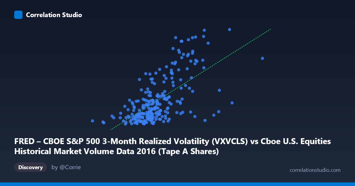
FRED – CBOE S&P 500 3-Month Realized Volatility (VXVCLS) vs Cboe U.S. Equities Historical Market Volume Data 2016 (Tape A Shares)
- Pearson correlation (r)
- 0.638
- Spearman correlation
- 0.619
- p-value
- 0
- Sample size (n)
- 252
- 95% confidence interval
- 0.5584 to 0.7059
- Granger causality
- None
- Granger optimal lag
- 1
- Time coverage
- 2016-01-04 to 2016-12-30
- Recomputed on refreshed data
- 2026-10-23 (r was 0.638)
AI analysis
Analysis: CBOE S&P 500 3-Month Realized Volatility vs. Tape A Share Volume (2016)
Relationship Overview The scatterplot reveals a moderate positive relationship between CBOE S&P 500 3-Month Realized Volatility (VXVCLS) and Tape A share volume on U.S. equities exchanges throughout 2016. As realized volatility increases, trading volume tends to rise as well — a pattern consistent with well-established market microstructure theory, where uncertainty and price discovery drive higher participation. The linear regression equation (y = 3.30×10⁻⁸x + 9.28) confirms this positive slope, indicating that each unit increase in volatility corresponds to a meaningful uptick in share volume. However, the relationship is clearly not perfectly linear, and the scatter around the regression line is substantial, suggesting that volatility alone is far from a complete explanation of trading activity.
Correlation Strength and Statistical Interpretation The Pearson correlation of r = 0.638 indicates a moderate-to-strong positive association, but the more telling statistic is r² = 0.407 — meaning realized volatility explains only about 40.7% of the variance in Tape A share volume. While statistically significant (p ≈ 0, n = 252, N = 3,622), this leaves nearly 60% of volume variation unexplained by volatility alone. The 95% confidence interval for r of [0.558, 0.706] is reassuringly narrow, indicating the estimate is stable and not an artifact of sampling. Crucially, the Granger causality tests show no significant predictive directionality in either direction (X→Y: F = 0.549, p = 0.459; Y→X: F = 0.828, p = 0.364). This means that knowing yesterday's volatility does not statistically help predict today's volume (and vice versa), which tempers any causal narrative — the correlation reflects co-movement, not a predictive lead-lag relationship at this one-period lag.
Patterns, Clusters, and Outliers Several notable structural features emerge from the data. The bulk of observations cluster in a relatively tight band — roughly volatility values between 14–20 and volume between 200M–320M shares — forming a dense core consistent with normal 2016 market conditions. However, there is a visually distinct upper-right cluster of outliers with volatility readings exceeding 22–27 and correspondingly elevated volumes (300M–450M+ shares). These high-volatility, high-volume points appear to follow a steeper relationship than the overall regression line, suggesting a possible non-linear or threshold effect at elevated stress levels. A handful of points with high volume but only moderate volatility (and vice versa) also deviate substantially from the fit, hinting at heteroscedasticity — variance in volume appears to fan out as volatility increases.
Confounding Factors and Caveats Several important caveats apply. First, the axes are swapped from their intuitive roles — the dataset notes indicate VXVCLS is plotted on the X-axis but is labeled as the Y-axis source variable and vice versa, which warrants verification before drawing directional conclusions. Second, 2016 was a uniquely event-driven year (Brexit in June, U.S. Presidential Election in November), and those episodic spikes likely drive much of the high-volatility cluster, making the relationship partially a product of specific macro shocks rather than a generalizable structural link. Third, Tape A share volume covers only NYSE-listed securities, and institutional routing decisions, ETF rebalancing flows, and index reconstitutions could independently affect volume independent of volatility. Finally, both variables are daily time-series data, and the absence of Granger causality at lag-1 does not rule out longer-lag dependencies or non-linear predictive structures.
Actionable Insights and Further Investigation Practitioners using volatility as a signal for expected liquidity conditions should be cautious: while the positive association is real, the unexplained 59% variance means volatility-based volume forecasts will carry substantial error. Segmenting the data by market regime (e.g., pre/post-Brexit, pre/post-election) would clarify whether the high-volatility outlier cluster represents a distinct regime with its own dynamics. Testing non-linear specifications (e.g., piecewise regression with a breakpoint around VXVCLS = 22) could significantly improve model fit given the apparent threshold behavior. Additionally, incorporating VIX term structure data, options open interest, or macroeconomic surprise indices as covariates could help explain the remaining variance and better isolate the true volatility-volume relationship from confounding event-driven dynamics.
X dataset: Cboe U.S. Equities Historical Market Volume Data 2016
Y dataset: FRED – CBOE S&P 500 3-Month Realized Volatility
Part of experiment: Daily - Cboe U.S. Equities Historical Market Volume Data 2016 vs FRED – CBOE S&P 500 3-Month Realized Volatility