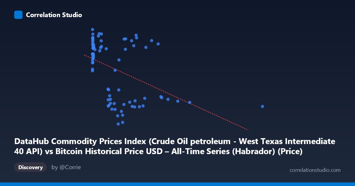
DataHub Commodity Prices Index (Crude Oil petroleum - West Texas Intermediate 40 API) vs Bitcoin Historical Price USD – All-Time Series (Habrador) (Price)
- Pearson correlation (r)
- -0.4501
- Spearman correlation
- -0.3834
- p-value
- 0.00002
- Sample size (n)
- 83
- 95% confidence interval
- -0.6068 to -0.2596
- Granger causality
- None
- Granger optimal lag
- 1
AI analysis
Analysis: Bitcoin Price vs. Commodity Price Index
1. Relationship Overview
The scatterplot displays a moderate negative relationship between the crude oil/commodity price index (X) and Bitcoin price (Y). Data points cluster heavily at low X values (under 300), with Y values ranging broadly from ~30 to ~110 in this region, while a sparser tail of higher X values (500–2452) tends to correspond to lower Y values. This creates the visual impression of a downward-sloping trend, though the density is highly uneven across the X range.
2. Strength, Direction, and Statistical Confidence
The correlation coefficient (r = -0.4501) indicates a moderate negative linear relationship, with R² = 0.2025 meaning only about 20% of the variance in Bitcoin price is explained by the commodity index — leaving 80% attributable to other factors. The 95% CI [-0.607, -0.260] excludes zero, and the p-value (1.966E-05) is highly significant, confirming this correlation is not due to random chance in this sample. However, statistical significance should not be conflated with practical strength: a moderate r² means this variable alone is a weak predictor. Critically, the Granger causality tests show no significant predictive direction in either direction (X→Y: p=0.166; Y→X: p=0.239). This means that despite the contemporaneous correlation, past values of one series do not meaningfully help forecast future values of the other — the relationship is likely coincidental co-movement or driven by a shared external factor, not a lead-lag causal dynamic.
3. Notable Patterns and Outliers
The data reveals a distinct clustering pattern rather than a smooth linear trend: a dense cloud of points at low X (0–50) with Y values spanning both high (~85-110) and low (~75-95) — suggesting these early/low-index points may represent an early Bitcoin era with its own volatility unrelated to commodity prices. A second, sparser cluster appears at mid-range X (200–700) with lower Y values (~40-60), and a few high-leverage outliers at very high X (997–2452) also show low Y. This non-uniform distribution suggests the "correlation" may be partly an artifact of temporal ordering (early Bitcoin history coinciding with certain oil price regimes) rather than a genuine functional relationship — the pattern looks more like two separate regimes than one continuous linear trend.
4. Confounding Factors and Caveats
Since this is time-series data spanning 2010–2017, both variables are likely non-stationary and trending over time, which can produce spurious correlations even with no causal link — the Granger test results support this concern. Bitcoin's price during this period was driven by adoption cycles, exchange launches, regulatory news, and speculative bubbles (e.g., 2013, 2017 rallies), while commodity/oil prices responded to OPEC decisions, global demand, and the 2014-2016 oil price collapse — largely independent macro drivers. The uneven sampling density (heavy clustering at low X) also means the regression line is disproportionately influenced by a small number of high-X outliers, and n=83 is a fairly small subsample of the full 449-point population, raising external validity concerns.
5. Recommendations for Further Investigation
Given the lack of Granger causality, this correlation should not be used for predictive trading or forecasting purposes. Further analysis should: (a) test for cointegration or apply differencing/detrending to rule out spurious correlation from shared time trends, (b) segment the analysis by distinct time periods or Bitcoin market regimes (early-stage vs. post-2013 bull run) to see if the relationship is regime-specific, (c) investigate potential confounders like USD strength, global risk sentiment, or macroeconomic indicators (e.g., VIX, interest rates) that could simultaneously affect both oil and Bitcoin prices, and (d) increase sample density in the underrepresented high-X range to verify whether the negative slope holds or is an artifact of sparse, high-leverage points.
X dataset: Bitcoin Historical Price USD – All-Time Series (Habrador)
Y dataset: DataHub Commodity Prices Index
Part of experiment: Bitcoin - Bitcoin Historical Price USD – All-Time Series (Habrador) vs DataHub Commodity Prices Index