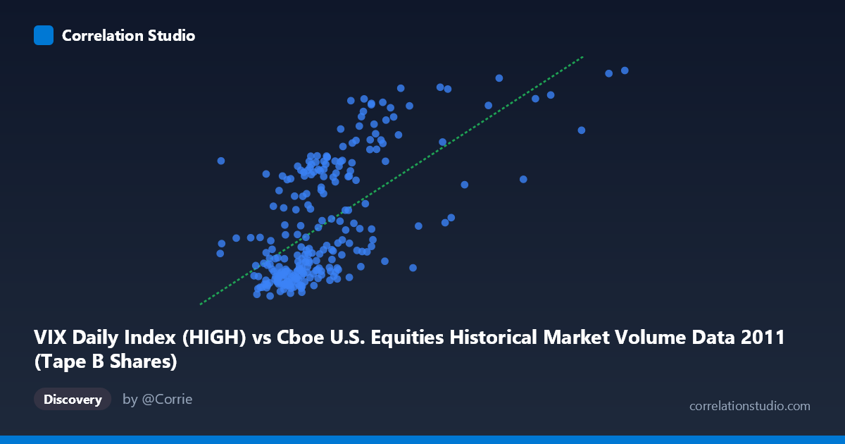
VIX Daily Index (HIGH) vs Cboe U.S. Equities Historical Market Volume Data 2011 (Tape B Shares)
- Pearson correlation (r)
- 0.6411
- Spearman correlation
- 0.6432
- p-value
- 0
- Sample size (n)
- 252
- 95% confidence interval
- 0.562 to 0.7085
- Granger causality
- None
- Granger optimal lag
- 1
AI analysis
Scatterplot Analysis: VIX Daily Index (HIGH) vs. Tape B Shares (2011)
Overall Relationship The scatterplot reveals a moderate positive relationship between the VIX Daily Index High values and Cboe U.S. Equities Tape B Share volume during 2011. As VIX High readings increase, Tape B share volume tends to rise correspondingly, which is intuitively consistent with market microstructure theory: elevated volatility typically drives heightened trading activity across equity venues. The linear regression equation (y = 1.71063E-07x + 8.607) confirms this positive slope, suggesting that for every unit increase in VIX High, Tape B shares increase proportionally, though with considerable scatter around the fitted line.
Correlation Strength and Statistical Significance The correlation coefficient of r = 0.641 indicates a moderate-to-strong positive association, with r² = 0.411 meaning that approximately 41.1% of the variance in Tape B shares is explained by VIX High values — a meaningful but incomplete explanation, leaving nearly 59% of variance attributable to other factors. The 95% confidence interval [0.562, 0.709] is reasonably tight and does not approach zero, and the p-value of effectively 0 confirms this result is highly statistically significant across the full population of N = 3,780 trading observations. However, the Granger causality tests tell a sobering story: neither direction (X→Y: F = 0.116, p = 0.734; Y→X: F = 0.114, p = 0.736) achieves significance at even relaxed thresholds. This means that while VIX and Tape B shares are contemporaneously correlated, neither variable reliably predicts the other at a one-period lag — the relationship is associative, not temporally predictive under this framework.
Notable Patterns, Clusters, and Outliers The data exhibit several visually distinct features. There is a dense cluster of observations concentrated in the lower-left region, where VIX High values fall roughly between 60–100 million and Tape B shares range from approximately 15–22 units, suggesting that calm, low-volatility trading days dominate the 2011 calendar — consistent with periods outside the summer/fall stress episodes. A secondary, more dispersed cluster appears in the upper-middle range, corresponding to elevated VIX periods. Several prominent outliers are visible in the upper-right quadrant (e.g., points near VIX High ~190M with Tape B ~43, and ~265M with extreme Y values), likely corresponding to the August 2011 U.S. debt ceiling crisis and European sovereign debt contagion, which drove historic VIX spikes. These high-leverage outliers may be disproportionately inflating the correlation coefficient.
Confounding Factors and Caveats Several important caveats warrant caution. First, 2011 was an atypical year marked by discrete macro stress events (August debt downgrade, Euro crisis), meaning the correlation may be regime-specific rather than structural. Second, the apparent relationship may be driven largely by a handful of extreme-volatility days — removing outliers could substantially weaken r. Third, there is a potential axis labeling inconsistency: the X-axis is described as VIX High from a market volume dataset, while the Y-axis draws Tape B Shares from a VIX dataset, suggesting possible dataset joining artifacts that should be verified. Fourth, both variables may respond simultaneously to a common driver (e.g., macro news shocks), making the correlation spurious in a causal sense — precisely what the Granger non-causality result implies.
Actionable Insights and Further Investigation Given these findings, practitioners and analysts should consider several next steps. Regime-segmented analysis — separating calm periods (VIX < 20) from stress periods (VIX 30) — would clarify whether the correlation holds uniformly or is driven by tail events. Rolling correlation windows across months would reveal whether the relationship strengthened during the August–October 2011 stress period specifically. Incorporating additional volume variables (Tape A, Tape C, total notional) alongside VIX could help decompose the 59% unexplained variance. Finally, exploring non-linear models (e.g., piecewise regression or threshold models) may better capture the apparent clustering behavior visible in the scatterplot, and testing longer Granger lags beyond one period could uncover delayed predictive dynamics not captured by the optimal lag-1 specification.
X dataset: Cboe U.S. Equities Historical Market Volume Data 2011
Y dataset: VIX Daily Index
Part of experiment: Daily - Cboe U.S. Equities Historical Market Volume Data 2011 vs VIX Daily Index