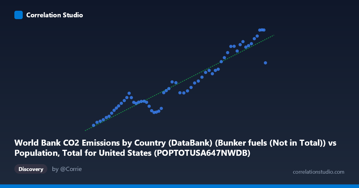
World Bank CO2 Emissions by Country (DataBank) (Bunker fuels (Not in Total)) vs Population, Total for United States (POPTOTUSA647NWDB) (POPTOTUSA647NWDB)
- Pearson correlation (r)
- 0.9501
- Spearman correlation
- 0.9371
- p-value
- 0
- Sample size (n)
- 61
- 95% confidence interval
- 0.9179 to 0.9699
- Granger causality
- None
- Granger optimal lag
- 10
- Time coverage
- 1960-01-01 to 2020-01-01
AI analysis
Scatterplot Analysis: U.S. Population vs. CO₂ Bunker Fuel Emissions (1960–2020)
1. Overall Relationship
The scatterplot reveals a strong, positive, and largely linear relationship between total U.S. population and CO₂ emissions from bunker fuels (international shipping and aviation fuels not included in national totals) over the 1960–2020 period. As the U.S. population grew from roughly 181 million to 332 million, bunker fuel emissions climbed from approximately 367 to 1,592 thousand metric tons of CO₂. The data points trace a coherent upward arc across six decades, consistent with the linear regression equation y = 7.39×10⁻⁶x − 980.78, suggesting that each additional million people in the U.S. population corresponds to roughly 7.4 units of additional bunker fuel CO₂ emissions on average.
2. Correlation Strength, Direction, and Causality
The Pearson correlation of r = 0.9501 is exceptionally strong, and the coefficient of determination R² = 0.9027 indicates that approximately 90.3% of the variance in bunker fuel emissions is statistically explained by U.S. population size alone. The 95% confidence interval for r [0.917, 0.970] is narrow and sits entirely in high-correlation territory, and the p-value of effectively zero confirms this is not a chance association across the n = 61 paired annual observations. However, the Granger causality tests tell a critical story: neither direction (X→Y: F = 0.87, p = 0.57; Y→X: F = 0.83, p = 0.60) achieves statistical significance even at optimal lag 10, meaning that past values of population do not significantly predict future bunker emissions beyond what bunker emissions already predict about themselves, and vice versa. This decisively separates statistical correlation from temporal predictive causation — the two variables co-move strongly but neither demonstrably drives the other in a lead-lag sense.
3. Notable Patterns, Clusters, and Outliers
The data broadly clusters into two visually distinguishable regimes: a lower-population, lower-emission cluster (population < ~250 million, roughly pre-1990) where data points are more densely packed and emissions increase modestly, and a higher-population, higher-emission region (post-~290 million) where the relationship steepens noticeably and scatter increases. One conspicuous outlier is the point at approximately (331.6M population, 1,168 CO₂) — the highest population value in the dataset yet with emissions well below the trend line, sitting roughly 400 units beneath what the regression predicts. This single point, likely corresponding to 2019 or 2020, is a meaningful deviation potentially reflecting COVID-19-era aviation and shipping collapse. A secondary cluster around the 300–330M range shows elevated variability, suggesting that the linear model's predictive power weakens somewhat at the higher population end.
4. Confounding Factors and Interpretive Caveats
The most fundamental caveat is that both variables are primarily time-driven — they each trend upward across the same six-decade span, making spurious correlation through shared temporal trend a near-certainty. This is precisely what the Granger test flags: the relationship is likely a coincident trend correlation rather than a mechanistic one. Bunker fuel emissions reflect international aviation and maritime activity, which is driven far more directly by globalization, trade volumes, fuel prices, aircraft efficiency improvements, and geopolitical shocks than by domestic population size per se. Population growth itself is an aggregate measure masking compositional shifts in age, urbanization, and consumption patterns. Additionally, with N = 65 total observations and n = 61 paired, there is limited degrees-of-freedom to detect complex non-linear dynamics, and autocorrelation within annual time series data can artificially inflate the apparent correlation and deflate p-values.
5. Actionable Insights and Further Investigation
Given the extremely high R² but failed Granger causality, the most productive next step would be to partial out the time trend by regressing both variables on year first and testing whether the residuals remain correlated — if they do not, the correlation is entirely spurious. Researchers should also incorporate direct economic drivers of bunker fuel demand (GDP, trade volume, jet fuel prices, fleet efficiency indices) in a multivariate model to test whether population retains explanatory power after controlling for these mediators. The anomalous low-emission, high-population outlier warrants isolation and flagging as a potential structural break point (likely 2020), and segmented regression or piecewise modeling should be evaluated given the apparent regime shift around the 290M population threshold. Finally, running this same analysis with per-capita bunker emissions as the Y variable would immediately test whether the population relationship is substantive or merely a scaling artifact — if per-capita emissions show no trend, the correlation here is almost certainly driven entirely by the shared upward temporal trajectory.
X dataset: Population, Total for United States (POPTOTUSA647NWDB)
Y dataset: World Bank CO2 Emissions by Country (DataBank)
Part of experiment: Yearly - Population, Total for United States (POPTOTUSA647NWDB) vs World Bank CO2 Emissions by Country (DataBank)