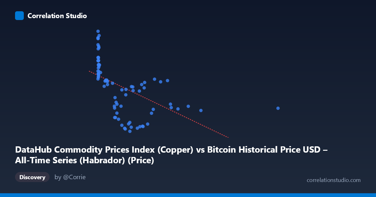
DataHub Commodity Prices Index (Copper) vs Bitcoin Historical Price USD – All-Time Series (Habrador) (Price)
- Pearson correlation (r)
- -0.5411
- Spearman correlation
- -0.769
- p-value
- 0
- Sample size (n)
- 83
- 95% confidence interval
- -0.6777 to -0.3683
- Granger causality
- None
- Granger optimal lag
- 10
AI analysis
Analysis: Copper Price Index vs. Bitcoin Historical Price
1. What the Visualization Reveals
The scatterplot shows a downward-sloping relationship between the copper commodity index (X) and Bitcoin price (Y), but the pattern is distinctly non-linear. Rather than a uniform linear decline, the data shows a steep drop-off in Y values as X increases from near-zero to roughly 300–500, followed by a much flatter, noisier relationship at higher X values (500–2452). This suggests the relationship is better characterized as a decaying curve (logarithmic or power-law) than a straight line, consistent with the note that Spearman's ρ exceeds Pearson's r.
2. Strength, Direction, and Uncertainty
The Pearson correlation (r = -0.5411) indicates a moderate negative linear association, with r² = 0.2927 meaning only ~29% of the variance in Y is explained by X under a linear model — the majority of variation (71%) is driven by other factors. The 95% CI [-0.6777, -0.3683] is reasonably tight and entirely negative, and the p-value (1.29e-07) confirms this correlation is highly unlikely due to chance in this sample. However, the Granger causality tests show no significant predictive direction in either direction (X→Y: p=0.80; Y→X: p=0.30) at a 10-period lag. This is a critical caveat: despite the statistically significant cross-sectional correlation, there is no evidence that movements in copper prices temporally precede or predict Bitcoin price movements, or vice versa. This strongly suggests the correlation is not causal and may instead reflect a shared trend, confound, or spurious co-movement over the 2010–2017 window.
3. Notable Patterns and Outliers
A dense cluster of points sits at very low X values (X < 20) with high, variable Y values (7,300–9,880) — this corresponds to Bitcoin's early history when copper index readings were near a floor/baseline. As X increases past ~100–300, Y drops sharply into the 5,000–7,000 range, and by X 700, Y stabilizes in a narrower 5,500–7,300 band with much weaker dependence on X. This creates an L-shaped or hyperbolic-decay pattern rather than a linear one. There are no extreme statistical outliers, but the high-Y/low-X cluster disproportionately influences the linear fit and inflates the apparent negative slope.
4. Confounding Factors and Caveats
The most important confound is time itself: Bitcoin price and the copper index are both time series spanning 2010–2017, and both may be trending due to independent macro factors (Bitcoin's adoption-driven exponential growth; copper's commodity supercycle dynamics) rather than any direct economic link. Since n=83 is a paired subsample of a larger population (N=449), sampling/aggregation choices (e.g., monthly averaging) could also distort the relationship. Additionally, pairing a commodity index with an asset price mismatches asset classes with different volatility regimes and drivers (industrial demand vs. speculative/adoption cycles), making a genuine economic relationship implausible without a strong theoretical basis.
5. Actionable Insights
Given the lack of Granger causality, this correlation should not be used for predictive or trading purposes — it likely reflects coincidental co-trending rather than a genuine driver-response relationship. For further investigation: (a) refit using a log-transform of X (or both variables) to test the suspected non-linear/logarithmic form and compare R² improvement; (b) detrend both series (e.g., differencing or removing time trend) before re-testing correlation, to isolate any genuine co-movement from shared drift; (c) test structural breaks/regime splits (e.g., pre/post 2013 Bitcoin bull run) since the relationship visibly differs across X ranges; and (d) consider alternative Bitcoin-relevant covariates (interest rates, USD index, trading volume) rather than copper prices, which lack a clear economic rationale for driving Bitcoin valuation.
X dataset: Bitcoin Historical Price USD – All-Time Series (Habrador)
Y dataset: DataHub Commodity Prices Index
Part of experiment: Bitcoin - Bitcoin Historical Price USD – All-Time Series (Habrador) vs DataHub Commodity Prices Index