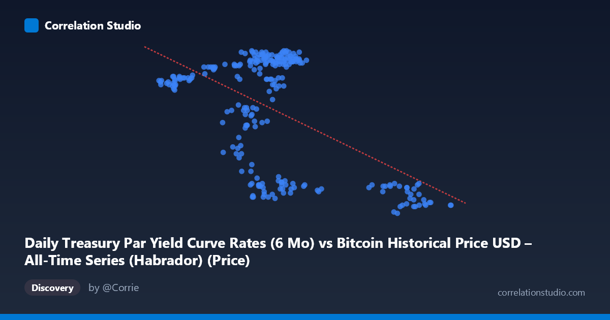
Daily Treasury Par Yield Curve Rates (6 Mo) vs Bitcoin Historical Price USD – All-Time Series (Habrador) (Price)
- Pearson correlation (r)
- -0.5467
- Spearman correlation
- -0.2041
- p-value
- 0
- Sample size (n)
- 250
- 95% confidence interval
- -0.6282 to -0.4534
- Granger causality
- None
- Granger optimal lag
- 1
- Time coverage
- 2024-01-02 to 2024-12-31
- Recomputed on refreshed data
- 2026-10-24 (r was -0.5467)
AI analysis
Analysis: Treasury 6-Month Yield vs. Bitcoin Price
Note on axis labeling: The metadata appears swapped — the X-axis values (39,507–105,990) with mean 65,880 are clearly Bitcoin prices in USD, while the Y-axis values (4.24–5.44) are clearly Treasury yield percentages. The analysis below interprets the data accordingly (X = Bitcoin price, Y = 6-month T-bill yield).
1. Relationship Overview
The scatterplot reveals a moderate negative relationship between Bitcoin price and the 6-month Treasury yield. As Bitcoin prices rise, yields tend to fall, though the relationship is far from a tight linear band — there's substantial scatter and evidence of clustering rather than a smooth continuous trend.
2. Strength, Direction, and Statistical Confidence
The correlation coefficient (r = -0.547) indicates a moderate negative association, with r² = 0.299 meaning only about 30% of the variance in Treasury yields is explained by Bitcoin price (or vice versa) — leaving 70% unexplained by this simple linear relationship. The 95% CI [-0.628, -0.453] is reasonably tight and excludes zero, and the p-value of ~0 confirms this correlation is statistically robust across the 250-day sample, not a fluke of noise. However, statistical significance with large N is easy to achieve even for modest effect sizes — the practical predictive power remains limited. Critically, the Granger causality tests show no significant predictive direction in either direction (Bitcoin→Yield: p=0.61; Yield→Bitcoin: p=0.27). This strongly suggests the correlation is not causal in a temporal/predictive sense — neither series reliably leads the other day-to-day. This is a classic case of contemporaneous correlation without lead-lag predictability, likely driven by a shared external factor rather than one variable driving the other.
3. Notable Patterns and Clusters
The data shows distinct clustering rather than a continuous linear spread: a dense cluster of points where yields sit high (5.2–5.44%) with Bitcoin prices in the ~57,000–70,000 range, and a separate cluster where yields drop to 4.2–4.5% with Bitcoin prices much higher (~87,000–101,000) or occasionally lower (~63,000–69,000 with yield ~4.3–4.5, suggesting a regime shift over time rather than a pure price-yield relationship). This bimodal/regime-like structure suggests the relationship may reflect two distinct macro periods (e.g., a rate-cutting cycle) rather than a smooth causal curve — consistent with time-series data where yield policy regimes shifted while Bitcoin also trended upward independently.
4. Confounding Factors and Caveats
Since this compares a daily macro policy variable (Treasury yields, which move via Fed policy decisions) against a speculative asset price (Bitcoin), the correlation is almost certainly confounded by broader macroeconomic conditions — Fed rate-cut expectations, inflation data, risk-on/risk-off sentiment, and liquidity conditions likely drive both series simultaneously. Both series are also non-stationary trending time series over the same calendar year (2024), so spurious correlation from shared trends (yields declining as part of a cutting cycle while Bitcoin rallied through its own bull cycle) is highly plausible. The lack of Granger causality reinforces that this is likely a shared-trend artifact rather than a genuine bidirectional economic relationship.
5. Suggested Further Investigation
Given the non-stationarity concerns, analysts should test both series for unit roots and consider differencing or detrending before re-assessing correlation (to rule out spurious trend-driven correlation). It would also be valuable to test correlation against other yield tenors (2Y, 10Y) and macro variables (DXY, real rates, Fed funds futures) to identify the true common driver. Given the regime-like clustering, segmenting the analysis by sub-periods (e.g., pre/post rate-cut announcements) could reveal whether the relationship strengthens or disappears within stable regimes. Finally, since Granger tests show no lead-lag structure, this pair should not be used for short-term predictive trading signals — it's better suited as a descriptive macro-correlation indicator than a forecasting tool.
X dataset: Bitcoin Historical Price USD – All-Time Series (Habrador)
Y dataset: Daily Treasury Par Yield Curve Rates
Part of experiment: Bitcoin - Bitcoin Historical Price USD – All-Time Series (Habrador) vs Daily Treasury Par Yield Curve Rates