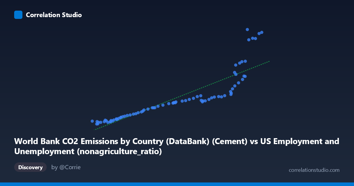
World Bank CO2 Emissions by Country (DataBank) (Cement) vs US Employment and Unemployment (nonagriculture_ratio)
- Pearson correlation (r)
- 0.8736
- Spearman correlation
- 0.9902
- p-value
- 0
- Sample size (n)
- 80
- 95% confidence interval
- 0.8092 to 0.9173
- Granger causality
- None
- Granger optimal lag
- 10
AI analysis
Scatterplot Analysis: Cement CO2 Emissions vs. US Non-Agriculture Employment Ratio
1. Overview of the Relationship
The scatterplot reveals a strong positive association between World Bank cement CO2 emissions and the US non-agriculture employment ratio, spanning annual observations from 1941 to 2020. As cement emissions increase along the x-axis (ranging from ~41,250 to ~155,113 units), the non-agriculture employment ratio rises substantially along the y-axis (from ~78 to ~2,609). However, the relationship is visibly non-linear: the data points trace a curve that starts relatively flat at lower emission values and accelerates sharply upward at higher values — particularly above ~130,000 on the x-axis — suggesting an exponential or power-law growth pattern rather than a simple linear one.
2. Correlation Strength, Direction, and Temporal Causality
The Pearson correlation of r = 0.8736 indicates a strong positive relationship, and the R² of 0.7632 means that approximately 76.3% of the variance in the non-agriculture employment ratio is statistically explained by cement CO2 emissions within this linear model. The 95% confidence interval of [0.8092, 0.9173] is relatively narrow and sits well above zero, confirming the estimate is robust. The p-value of effectively 0 rules out chance as an explanation for this association. That said, the Granger causality tests show no significant predictive direction in either direction (X→Y: F = 0.378, p = 0.950; Y→X: F = 0.921, p = 0.523), meaning that past values of cement emissions do not reliably forecast future non-agriculture employment ratios, and vice versa. This is a critical caveat: the variables move together over time, but neither appears to drive the other in a temporal, predictive sense — strongly implying a shared underlying driver (likely broad economic or industrial growth) rather than a direct causal mechanism.
3. Notable Patterns, Clusters, and Outliers
The data cluster into two visually distinct regimes. The lower-left cluster (x < ~110,000; y < ~850) is dense and relatively tightly packed, representing what are likely mid-20th-century observations where both metrics were lower and variance was modest. The upper-right region (x ~130,000; y ~1,000) shows dramatically increasing spread and several high-leverage points — including observations near (145,446; 2,608), (153,336; 2,502), and (155,113; 2,533) — that deviate substantially above the linear regression line. These extreme values are consistent with the Spearman ρ exceeding Pearson r, which the analysis flags as evidence of non-linearity. The linear regression equation (y = 0.0156x − 749.13) systematically underpredicts these high-end values, confirming the model is misspecified at the upper tail.
4. Confounding Factors and Interpretation Caveats
The most significant caveat is that both variables are likely proxies for overall long-run economic and industrial expansion in the United States and globally. Over the 1941–2020 period, GDP growth, population increase, urbanization, and industrialization would naturally push both cement production/emissions and non-agricultural employment upward simultaneously — creating a spurious or heavily confounded correlation. Additionally, temporal autocorrelation is almost certain in annual time-series data of this kind; consecutive years are not independent observations, which inflates the apparent statistical significance. The dataset label mismatch (cement CO2 from a World Bank dataset appearing in a US employment file, and vice versa) also warrants scrutiny — data provenance and unit definitions should be verified before drawing any inference. Finally, the non-linearity in the upper tail may reflect specific historical episodes (e.g., post-2000 Chinese cement boom) that are not representative of the underlying structural relationship.
5. Actionable Insights and Further Investigation
Given the non-linearity flag, a logarithmic or polynomial regression (e.g., y = a·ln(x) + b, or a quadratic model) should be fitted and compared against the linear model using AIC/BIC to determine whether it materially improves fit — particularly for the high-emission tail. Researchers should detrend both time series (e.g., by differencing or removing a common GDP/population trend) to test whether any residual correlation persists after accounting for the shared secular growth trend, which would help distinguish genuine co-movement from spurious correlation. Given the failed Granger causality in both directions, a vector autoregression (VAR) with exogenous controls (GDP, population, energy prices) would help isolate whether any direct relationship exists beyond the common trend. Finally, examining subperiod stability (pre/post-1980, pre/post-2000) would reveal whether the relationship has changed structurally over time, which would be valuable for both climate policy modeling and labor market forecasting contexts.
X dataset: US Employment and Unemployment
Y dataset: World Bank CO2 Emissions by Country (DataBank)
Part of experiment: Yearly - US Employment and Unemployment vs World Bank CO2 Emissions by Country (DataBank)