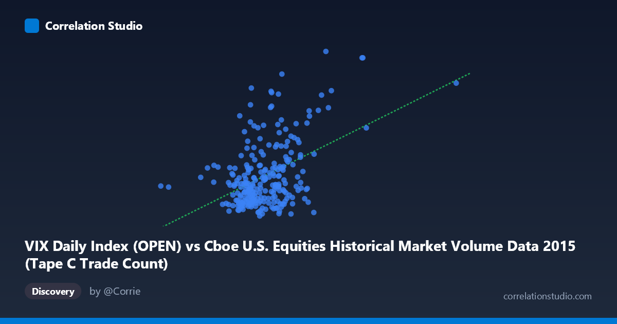
VIX Daily Index (OPEN) vs Cboe U.S. Equities Historical Market Volume Data 2015 (Tape C Trade Count)
- Pearson correlation (r)
- 0.4513
- Spearman correlation
- 0.2988
- p-value
- 0
- Sample size (n)
- 252
- 95% confidence interval
- 0.3471 to 0.5445
- Granger causality
- None
- Granger optimal lag
- 1
AI analysis
Scatterplot Analysis: VIX Open vs. Tape C Trade Count (2015)
Overall Relationship The scatterplot reveals a moderate positive relationship between the Cboe VIX Daily Index (Open) and Tape C Trade Count across U.S. equities exchanges in 2015. As the VIX opens at higher levels — signaling greater anticipated market volatility — Tape C trade counts tend to increase. This is conceptually intuitive: elevated fear or uncertainty in markets typically drives higher trading activity as participants rush to hedge, rebalance, or exit positions. The linear regression (y = 1.367×10⁻⁵x + 6.349) captures this upward trend, though the scatter around the regression line is substantial, immediately signaling that the relationship is real but far from deterministic.
Correlation Strength and Statistical Framing The Pearson correlation of r = 0.4513 indicates a moderate positive association, but the coefficient of determination tells a more sobering story: r² = 0.2037, meaning only about 20.4% of the variance in Tape C Trade Count is explained by VIX Open levels. The remaining ~80% of variation is driven by factors outside this bivariate model. The 95% confidence interval of [0.3471, 0.5445] is meaningfully above zero and relatively tight given n = 252, reflecting genuine statistical stability. The p-value of 4.752×10⁻¹⁴ is extraordinarily small, firmly rejecting the null hypothesis of no correlation — with N = 3,302 in the underlying population, this signal is robust. However, the Granger causality results offer an important corrective: neither direction (X→Y: F = 0.2556, p = 0.614; Y→X: F = 0.0174, p = 0.895) reaches significance at any conventional threshold. This means that while VIX and trade counts move together, neither variable temporally predicts the other at a one-period lag — the relationship is contemporaneous rather than predictive, limiting any practical forecasting utility derived from this correlation alone.
Notable Patterns, Clusters, and Outliers The sample points reveal several structural features worth noting. The bulk of observations cluster in the VIX range of roughly 600,000–900,000 (X-axis) with Y values between 12 and 20, forming a dense core. However, there are clear high-leverage outliers in the upper right: points such as (1,194,527, 31.13), (1,210,005, 22.55), and (954,355, 24.64) pull the regression line upward and likely inflate the correlation coefficient. There also appear to be outliers in the lower-right quadrant — notably (975,204, 12.20) and (825,366, 13.26) — where high trade volumes coincide with low VIX readings, breaking the expected pattern. This asymmetry suggests non-linearity or regime-dependent behavior: the relationship may strengthen considerably during high-volatility episodes (likely mid-2015 during the August market correction) while being nearly flat during calm periods. A piecewise or threshold regression model might better capture this structure than a single linear fit.
Confounding Factors and Interpretive Caveats Several confounds complicate a clean causal interpretation. First, both variables share a common driver — broad market stress events (e.g., the August 2015 China-driven selloff) simultaneously spike VIX and flood exchanges with volume, creating spurious co-movement that is more a reflection of shared external shocks than a direct causal link. Second, Tape C specifically covers NYSE Arca-listed securities, which may react differently to volatility than Tape A or B securities, introducing selection bias if generalized. Third, the VIX Open represents anticipated volatility at the start of the trading day; intraday dynamics or closing VIX levels might produce a different correlation structure. Fourth, secular trends within 2015 — such as exchange fee changes, algorithmic trading patterns, or ETF rebalancing cycles — could create spurious temporal correlation across the calendar year independent of volatility dynamics.
Actionable Insights and Further Investigation Despite the Granger non-result, this correlation has risk management utility when interpreted contemporaneously: on days when the VIX opens elevated, market participants and exchange operators should anticipate above-average Tape C trade counts, informing capacity planning and liquidity provisioning. For deeper investigation, several steps are warranted: (1) segment the analysis by volatility regime (e.g., VIX < 15, 15–20, 20) to test whether the correlation strengthens nonlinearly above a stress threshold; (2) introduce lagged macroeconomic or sentiment variables as controls to isolate the VIX-volume relationship from shared confounders; (3) extend Granger testing to longer lags (2–5 periods) in case one-period is too short to capture any predictive signal; and (4) compare Tape A and Tape B trade counts against the same VIX series to determine whether this relationship is exchange-specific or systemic. A multivariate model incorporating VIX, market returns, and bid-ask spreads would likely explain substantially more than the current 20.4% of variance.
X dataset: Cboe U.S. Equities Historical Market Volume Data 2015
Y dataset: VIX Daily Index
Part of experiment: Daily - Cboe U.S. Equities Historical Market Volume Data 2015 vs VIX Daily Index