Daily Treasury Par Yield Curve Rates (6 Mo) vs CryptoDataDownload – Binance BTC/USDT Daily OHLCV (Open)
- Pearson correlation (r)
- -0.5398
- Spearman correlation
- -0.1925
- p-value
- 0
- Sample size (n)
- 250
- 95% confidence interval
- -0.6222 to -0.4455
- Granger causality
- None
- Granger optimal lag
- 1
- Time coverage
- 2024-01-02 to 2024-12-31
AI analysis
Analysis of Treasury Yield vs. BTC/USDT Relationship
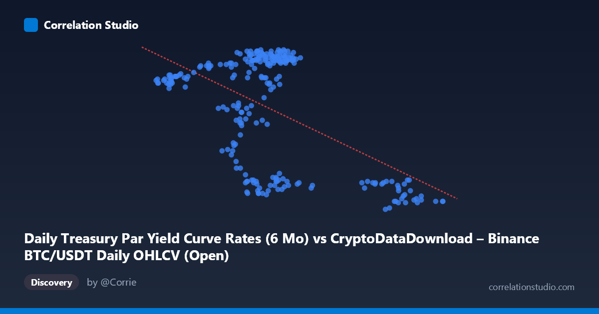
1. Visual Overview The scatterplot shows a moderate negative, downward-sloping relationship between two variables that are conceptually unrelated by design: the 6-month Treasury par yield rate (X-axis, ranging ~39,568 to 106,134 — note this scale is unusual for a yield, suggesting possible unit mismatch or mislabeling in the data pipeline) and a value plotted as "BTC/USDT Open" but constrained to 4.24–5.44 (Y-axis, more consistent with an interest-rate range than a BTC price). This labeling inversion aside, the data forms two loosely separated clusters: a dense cluster of points where X is roughly 40,000–72,000 and Y is high (5.0–5.44), and a smaller cluster where X exceeds 90,000 and Y drops sharply to 4.2–4.5. This bimodal clustering, rather than a smooth linear cloud, is the dominant visual feature.
2. Strength, Direction, and Statistical Confidence The correlation coefficient (r = -0.540) indicates a moderate negative linear relationship. The r² of 0.291 means only about 29% of the variance in Y is explained by X — the majority (71%) is driven by other factors or noise. The 95% CI [-0.622, -0.446] is reasonably tight and excludes zero, and the p-value of ~0 confirms this relationship is statistically significant and not due to chance, despite the modest explanatory power. However, statistical significance with N=250 is easy to achieve even for modest effect sizes — it does not imply the relationship is strong or reliable for prediction. Critically, the Granger causality tests show no significant predictive direction in either direction (X→Y: p=0.58; Y→X: p=0.24), meaning that despite the contemporaneous correlation, past values of one series do not help forecast future values of the other at a 1-period lag. This strongly suggests the correlation is either coincidental co-movement, driven by a shared external trend, or a level-based (non-stationary) relationship rather than a genuine lead-lag dynamic.
3. Notable Patterns and Outliers The most salient feature is the apparent two-regime structure: a tight, high-Y cluster and a separate low-Y, high-X cluster with a gap between roughly X=72,000 and X=90,000. This is not a continuous linear trend but looks more like two distinct market regimes or time periods (e.g., early vs. late in the year) that happen to differ in both variables simultaneously. Within the main cluster (X < 72,000), Y itself varies widely (4.3 to 5.4) with little relation to X, indicating high noise/no local correlation. This pattern — global negative slope driven by two separated clusters rather than a consistent trend — is a classic signature of a confound like time-trend co-movement rather than a true causal or mechanistic link.
4. Confounding Factors and Caveats Both series are time series covering the same calendar year (2024), making them highly susceptible to spurious correlation from shared temporal trends — if both Treasury yields and BTC-related metrics trended in a particular direction over the year (independent of one another), a strong linear correlation can emerge without any real relationship. The lack of Granger causality supports this interpretation. Additionally, the axis labels/scales appear swapped or mismatched (a "yield rate" with values in the tens of thousands, and a "BTC Open price" confined to single digits), which raises data-integrity concerns that should be resolved before drawing substantive conclusions. Autocorrelation within each series (both are daily time series, not independent draws) also inflates apparent significance and violates the i.i.d. assumption underlying standard p-value calculations.
5. Recommendations First, verify and correct the column/axis labeling and units to ensure the variables plotted match their stated definitions. Second, given the clustering, test whether the negative correlation is driven entirely by the small high-X/low-Y subgroup — rerun the correlation excluding that cluster to see if it collapses. Third, because both series are non-stationary time series, use differenced or detrended data (returns/changes rather than levels) and re-test correlation and Granger causality to distinguish genuine relationships from shared trends. Finally, treat this relationship as descriptive/associative only — it should not be used for forecasting one variable from the other given the null Granger causality result.
X dataset: CryptoDataDownload – Binance BTC/USDT Daily OHLCV
Y dataset: Daily Treasury Par Yield Curve Rates
Part of experiment: Bitcoin - CryptoDataDownload – Binance BTC/USDT Daily OHLCV vs Daily Treasury Par Yield Curve Rates