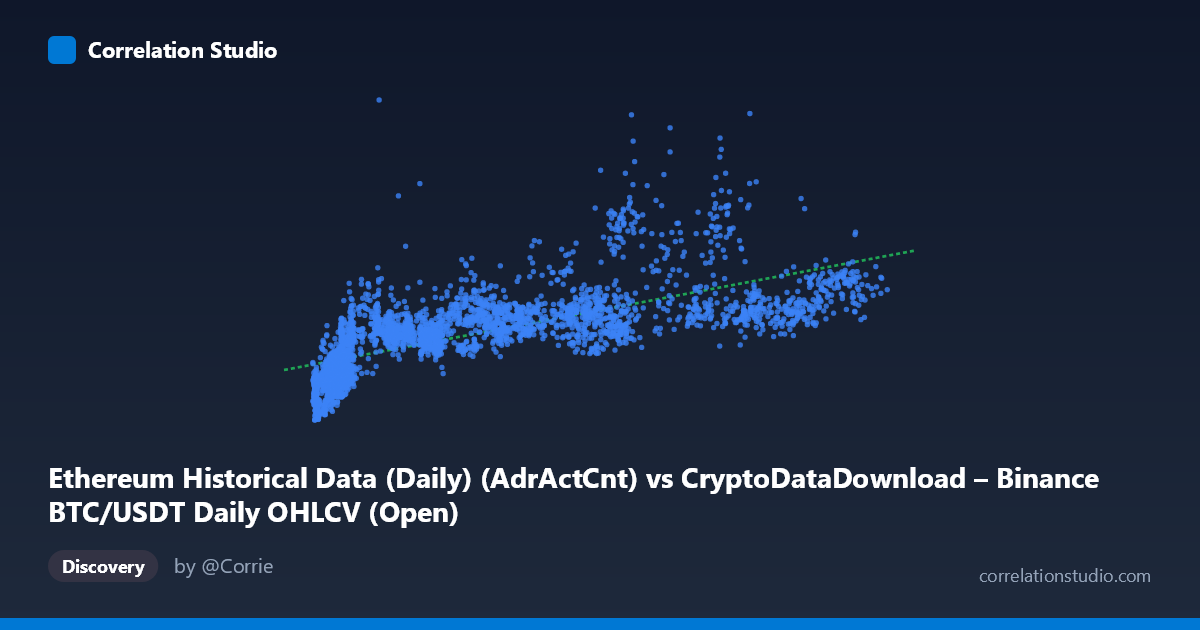
Ethereum Historical Data (Daily) (AdrActCnt) vs CryptoDataDownload – Binance BTC/USDT Daily OHLCV (Open)
- Pearson correlation (r)
- 0.6958
- Spearman correlation
- 0.8291
- p-value
- 0
- Sample size (n)
- 3191
- 95% confidence interval
- 0.6775 to 0.7133
- Granger causality
- None
- Granger optimal lag
- 10
- Time coverage
- 2017-08-17 to 2026-05-20
AI analysis
Analysis of the Scatterplot Relationship
1. What the Visualization Reveals
The scatterplot shows a positive, moderately strong association between the X variable (labeled here as Ethereum active address count, though the metadata is oddly mismatched with BTC/USDT OHLCV data) and Y (labeled as an Open price series). As X increases from roughly 3,000 to 125,000, Y tends to rise from the 130K–150K range toward values exceeding 900K–1.5M. The relationship is not a tight line — there's substantial vertical scatter at every X level, particularly in the low-to-mid X range (5,000–30,000), where Y values span from ~150,000 to over 600,000. This spread narrows somewhat at higher X values, where most points cluster between 500K and 1M.
2. Strength, Direction, and Uncertainty
The Pearson correlation (r = 0.696) indicates a moderate-to-strong positive linear relationship, with r² = 0.484 meaning the linear model explains only about 48% of the variance in Y — leaving over half unexplained by X alone. The 95% confidence interval [0.678, 0.713] is tight, and the p-value of ~0 confirms this correlation is highly statistically significant and not a product of chance, aided considerably by the large sample size (n = 3,191). However, statistical significance should not be conflated with practical strength: the moderate r² means X is a partial, not dominant, predictor of Y.
Critically, the Granger causality tests show no significant predictive direction in either direction (X→Y: p = 0.71; Y→X: p = 0.64) even at an optimal lag of 10 periods. This is an important caveat: despite the contemporaneous correlation, neither series helps forecast the other's future values based on past values. This suggests the relationship is likely driven by a shared external factor (e.g., overall crypto market sentiment, macro liquidity conditions) rather than one variable causing or leading the other.
3. Notable Patterns and Non-linearity
The note that Spearman ρ exceeds Pearson r is a strong signal that the true relationship is monotonic but non-linear — likely logarithmic or power-law in shape. This aligns with the visual pattern: rapid, steep increases in Y for small increases in X at low X values (e.g., X near 4,000–10,000 shows Y ranging widely from 150K to 500K+), followed by a flattening or slower marginal increase in Y as X grows large (X 80,000 shows Y plateauing around 500K–900K with some high outliers near 1.5M). This is classic diminishing-returns/log-shaped behavior, not a constant-slope linear one. There also appear to be a few high-leverage outliers (e.g., Y 900,000 at moderate X ~70,000–90,000) that may be pulling the linear fit.
4. Confounding Factors and Caveats
Several caveats limit causal interpretation: - Metadata mismatch: The axis labels reference different datasets (Ethereum active addresses vs. BTC/USDT OHLCV Open) that don't logically align with the described columns — this may indicate a data pipeline error or mislabeling that should be verified before drawing domain conclusions. - Time-series autocorrelation: Both series likely trend upward over the 2017–2026 window (bull market cycles), which can inflate correlation via shared time trends rather than genuine dependency. - Non-stationarity: Crypto prices and on-chain metrics are typically non-stationary; Granger tests and Pearson r are more reliable on differenced/detrended data. - Third-variable confounding: Overall crypto market cycles, BTC price movements, or macro liquidity conditions could independently drive both variables.
5. Actionable Insights
1. Verify data labeling — confirm the axis metadata (dataset/column names) are correctly mapped to avoid misinterpreting the relationship. 2. Re-fit with non-linear models — try log-log or log-linear regression given the Spearman/Pearson divergence; this will likely raise explained variance substantially. 3. Detrend/difference the series before re-running correlation and Granger tests to control for shared macro trends and test for a "real" leading indicator relationship. 4. Segment by market regime (bull vs. bear periods) to see if the relationship strength or shape changes across cycles. 5. Treat this as a co-movement, not a forecasting signal — given the null Granger results, do not use X to predict future Y (or vice versa) in a trading/predictive model without further validation.
X dataset: CryptoDataDownload – Binance BTC/USDT Daily OHLCV
Y dataset: Ethereum Historical Data (Daily)
Part of experiment: Bitcoin - CryptoDataDownload – Binance BTC/USDT Daily OHLCV vs Ethereum Historical Data (Daily)