Crude Oil Prices: West Texas Intermediate (WTI) - Cushing, Oklahoma (DCOILWTICO) | FRED | St. Louis Fed (DCOILWTICO) vs CryptoDataDownload – Binance BTC/USDT Daily OHLCV (Unix)
- Pearson correlation (r)
- 0.4381
- Spearman correlation
- 0.5028
- p-value
- 0
- Sample size (n)
- 2197
- 95% confidence interval
- 0.4037 to 0.4713
- Granger causality
- None
- Granger optimal lag
- 1
- Time coverage
- 2017-08-17 to 2026-06-25
- Recomputed on refreshed data
- 2026-10-22 (r was 0.4381)
AI analysis
Analysis: WTI Crude Oil Prices vs. BTC/USDT Time Index
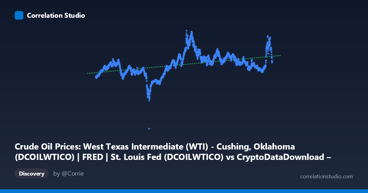
Note on axis labeling: The axis labels appear swapped in the metadata (X is labeled as OHLCV data, Y as WTI price), but based on the value ranges — X spans ~1.5–1.78 trillion (Unix millisecond timestamps) and Y spans -37 to 124 (plausible oil price range) — this appears to actually be a time-series plot of WTI crude oil prices (Y) against time (X), covering roughly 2017 to 2026.
1. What the Visualization Reveals
The scatterplot shows WTI crude oil prices plotted over an ~9-year span. Rather than depicting a relationship between two independent economic variables, this is essentially a price history chart. The data shows oil prices evolving from the mid-$50s (2017-2019), collapsing dramatically toward the 2020 negative-price event (Y approaches -37), then recovering and trending upward into the $80-120 range by 2022-2026, with continued volatility.
2. Strength, Direction, and Statistical Interpretation
The reported correlation (r = 0.438, r² = 0.192) indicates a moderate positive relationship between time and price — essentially confirming an upward secular trend in oil prices over the sample period. However, only 19.2% of price variance is explained by time alone, meaning the vast majority (81%) of price movement is driven by other factors (supply shocks, geopolitical events, demand cycles) not captured by a simple linear time trend. The tight confidence interval [0.404, 0.471] and p-value ≈ 0 confirm this trend is statistically robust and not due to chance, despite its modest explanatory power. The Granger causality results (p = 0.82 and p = 0.30) are unsurprising and largely a technical artifact here — since one variable is essentially a time index, standard Granger causality tests (which examine whether lagged values of one series predict another) are not meaningfully interpretable in this context. This result should be disregarded for substantive causal inference.
3. Notable Patterns and Outliers
The most striking feature is the 2020 negative-price outlier (Y = -36.98), reflecting the unprecedented COVID-19 storage crisis when WTI futures briefly traded below zero. Excluding this anomaly, the data shows distinct regimes: a relatively stable/low period (2017-2019, prices 40-70), a sharp trough (2020), a strong recovery and bull run (2021-2022, peaking above 100), and continued elevated volatility with values fluctuating between 60-120 through 2023-2026. The linear regression line (with a negative intercept extending to prehistoric dates) is a poor structural fit — the true pattern is non-linear/regime-based, with the low r² reflecting this mismatch between a straight-line model and a series driven by cyclical shocks.
4. Confounding Factors and Caveats
Critical caveats apply: (1) Time is not a causal variable — using it as a predictor only captures a generic trend, not underlying drivers like OPEC+ production decisions, geopolitical conflicts (e.g., Russia-Ukraine war), demand shifts, or macroeconomic cycles. (2) The linear model is inappropriate for data with clear structural breaks and volatility clustering. (3) The axis/dataset labeling inconsistency in the metadata raises data provenance concerns that should be resolved before drawing further conclusions. (4) Autocorrelation in time-series price data violates independence assumptions underlying standard correlation/significance tests, likely inflating apparent statistical confidence.
5. Recommendations
Given that this is fundamentally a price time series, more appropriate analyses would include: time-series decomposition (trend/seasonal/cyclical components), regime-switching models to capture the distinct pre-COVID, COVID-shock, and post-COVID phases, and volatility modeling (e.g., GARCH) given the evident heteroskedasticity. If the original intent was to compare crude oil prices to BTC/USDT trading data (as dataset descriptions suggest), the actual variables should be correctly re-plotted against each other (not against time) to test for genuine cross-asset relationships, with attention to potential spurious correlation from shared macro trends (e.g., both being risk assets sensitive to interest rates and inflation).
X dataset: CryptoDataDownload – Binance BTC/USDT Daily OHLCV
Y dataset: Crude Oil Prices: West Texas Intermediate (WTI) - Cushing, Oklahoma (DCOILWTICO) | FRED | St. Louis Fed
Part of experiment: Bitcoin - CryptoDataDownload – Binance BTC/USDT Daily OHLCV vs Crude Oil Prices: West Texas Intermediate (WTI) - Cushing, Oklahoma (DCOILWTICO) | FRED | St. Louis Fed