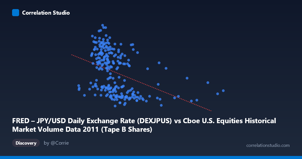
FRED – JPY/USD Daily Exchange Rate (DEXJPUS) vs Cboe U.S. Equities Historical Market Volume Data 2011 (Tape B Shares)
- Pearson correlation (r)
- -0.4056
- Spearman correlation
- -0.5195
- p-value
- 0
- Sample size (n)
- 250
- 95% confidence interval
- -0.5043 to -0.2965
- Granger causality
- None
- Granger optimal lag
- 1
AI analysis
Scatterplot Analysis: JPY/USD Exchange Rate vs. Cboe U.S. Equities Market Volume (2011)
1. Overall Relationship and Visualization The scatterplot reveals a modest negative relationship between U.S. equity market trading volume (X-axis, measured in shares) and the JPY/USD exchange rate (Y-axis, measured in yen per dollar). As trading volume increases, the yen tends to be weaker against the dollar (higher yen-per-dollar values correspond to a weaker yen). The data spans the full calendar year 2011, capturing a period of notable market turbulence including the Tōhoku earthquake/tsunami, the European debt crisis escalation, and the U.S. debt ceiling standoff. The scatter is broadly dispersed across the volume range, with the bulk of observations clustered between roughly 60–140 million shares and yen values between 76–84, suggesting the linear trend, while present, is far from dominant.
2. Correlation Strength, Direction, and Temporal Causality The Pearson correlation of r = −0.406 indicates a statistically significant but moderate negative association. Practically, however, the R² of 0.1645 means that only ~16.5% of the variance in the JPY/USD rate is explained by equity trading volume — the vast majority (~83.5%) of the exchange rate's movement is driven by factors entirely outside this model. The 95% confidence interval of [−0.504, −0.297] is meaningfully negative throughout, confirming the direction is reliable, and the p-value of 2.55 × 10⁻¹¹ makes this statistically indistinguishable from chance essentially impossible at conventional thresholds given N = 3,780. Despite this statistical significance, the Granger causality tests yield no significant predictive directionality in either direction (X→Y: F = 0.143, p = 0.706; Y→X: F = 0.198, p = 0.657). This is a critical distinction: while the two variables co-move to a degree, neither variable meaningfully predicts the other's future values at the one-period lag tested. The correlation is likely coincidental co-variation driven by shared macro conditions rather than any direct causal mechanism.
3. Notable Patterns, Clusters, and Outliers Several features stand out in the sample data. There is a notable cluster of high-volume days (120 million shares) that consistently correspond to lower yen values (76–78 JPY/USD), suggesting that extreme volume spikes — likely tied to crisis-driven selling or volatility events — coincided with a stronger yen, a classic safe-haven pattern. Conversely, the highest yen values (84–85 JPY/USD, indicating a weaker yen) tend to appear at moderate-to-low volume levels. The point at (265M shares, 77.53) is a clear high-leverage outlier at the far right of the X-axis, representing an exceptionally high-volume day that broadly conforms to the trend. The point at (78.2M shares, 85.26) represents the highest yen-per-dollar value in the sample — a notably low-volume, weak-yen day. The note that Spearman ρ exceeds Pearson r further suggests the relationship is better described as monotonic but non-linear, with diminishing returns at extreme volume values, potentially warranting a logarithmic or polynomial fit.
4. Confounding Factors and Interpretive Caveats Several confounds make this correlation difficult to interpret causally. 2011 was an unusually eventful year — the Tōhoku disaster in March triggered both sharp yen appreciation (safe-haven flows) and elevated market volatility/volume simultaneously, which could alone generate a spurious negative correlation. More broadly, both variables are driven by common macro factors: risk-off episodes tend to simultaneously spike U.S. equity volumes (panic selling) and strengthen the yen (safe-haven demand), producing correlation without direct causation. The axis assignment also warrants scrutiny — the dataset labels suggest X and Y may have been assigned non-intuitively (volume data labeled on the exchange rate axis and vice versa), which should be verified before drawing conclusions. Additionally, daily data introduces autocorrelation in both series, which can inflate statistical significance; the effective sample size may be considerably smaller than n = 250 or N = 3,780.
5. Actionable Insights and Further Investigation Given these findings, several follow-up analyses are warranted. First, test non-linear fits (logarithmic or polynomial) as suggested by the Spearman/Pearson divergence — the relationship may be threshold-driven, with the correlation concentrated in high-stress market regimes. Second, segment the data by market regime (e.g., pre/post-Tōhoku, high-VIX vs. low-VIX periods) to test whether the correlation is driven entirely by crisis episodes — if so, it is not a stable structural relationship. Third, extend the Granger causality test to multiple lags (e.g., 1–10 days) to rule out longer-horizon predictive relationships. Fourth, include a volatility index (VIX) as a mediating variable — it is plausibly the common driver of both series and including it may substantially reduce or eliminate the residual correlation. Finally, verify dataset axis alignment, as the column-to-axis assignment described in the metadata appears potentially transposed, which would affect all directional interpretations.
X dataset: Cboe U.S. Equities Historical Market Volume Data 2011
Y dataset: FRED – JPY/USD Daily Exchange Rate
Part of experiment: Daily - Cboe U.S. Equities Historical Market Volume Data 2011 vs FRED – JPY/USD Daily Exchange Rate