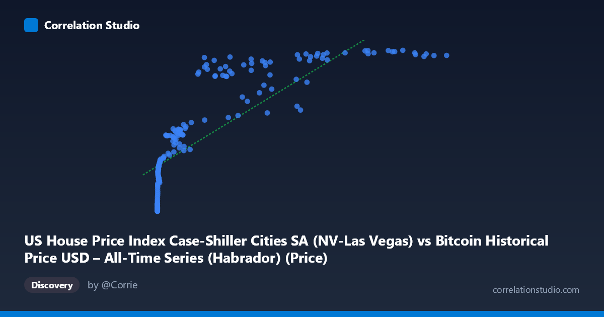
US House Price Index Case-Shiller Cities SA (NV-Las Vegas) vs Bitcoin Historical Price USD – All-Time Series (Habrador) (Price)
- Pearson correlation (r)
- 0.821
- Spearman correlation
- 0.9683
- p-value
- 0
- Sample size (n)
- 189
- 95% confidence interval
- 0.7682 to 0.8626
- Granger causality
- None
- Granger optimal lag
- 9
- Time coverage
- 2010-08-01 to 2026-04-01
- Recomputed on refreshed data
- 2026-10-22 (r was 0.8164)
AI analysis
Analysis: Bitcoin Price vs. Las Vegas Case-Shiller Home Price Index
1. What the Visualization Reveals
The scatterplot shows a strong positive association between Bitcoin's USD price and the Las Vegas Case-Shiller Home Price Index, but the shape of that relationship is distinctly non-linear. At low Bitcoin prices (under ~$1,000), the index values cluster tightly between 90–160, rising steeply on a compressed X-axis. As Bitcoin prices climb into the tens of thousands, the index values plateau and compress into a narrower band (roughly 270–305), producing a curve that looks logarithmic rather than a straight diagonal line. This is a classic signature of two independent variables that both trended upward over the same calendar period rather than variables mechanically driving one another.
2. Strength, Direction, and Uncertainty
The Pearson correlation (r = 0.8164, r² = 0.6665) indicates a strong positive linear relationship, with about 67% of the variance in the housing index "explained" by Bitcoin price in a naive linear model. The 95% CI [0.762, 0.859] is tight and the p-value is effectively zero, so the correlation is not a statistical fluke — it's a robust, reproducible pattern in this sample. However, statistical significance here should not be conflated with causal or economically meaningful linkage. The Granger causality tests are decisive on this point: neither direction shows predictive power (X→Y: p=0.752; Y→X: p=0.782). This means past Bitcoin prices do not help forecast future housing index values, or vice versa — the correlation is almost certainly driven by both series co-trending over time (2010–2026) rather than one causing the other.
3. Notable Patterns and Outliers
Several features stand out: - Curvature/saturation: The index appears to approach an asymptote near 300–305 as Bitcoin prices exceed $60,000, while Bitcoin continues to range widely up to $118,670 — suggesting a log-linear or power relationship would fit better (consistent with the note that Spearman ρ Pearson r). - Low-end density: A large cluster of points sits at very low Bitcoin prices ($0.06–$20) corresponding to the earliest years (2010–2013), where the housing index was still recovering from the 2008 crash (values ~90–107). - Mid-range volatility: Between $20,000–$60,000, index values show more scatter (e.g., 215–293), reflecting Bitcoin's boom-bust cycles (2021 crash, 2022 bear market) occurring while housing prices moved more smoothly. - No extreme single-point outliers dominate; the pattern is a smooth curve with expected noise.
4. Confounding Factors and Caveats
This is a textbook case of spurious correlation via shared time trend. Both series are non-stationary time series that generally rose from 2010–2026 due to entirely different macro drivers: Bitcoin's price is driven by crypto adoption, speculation, and liquidity cycles, while the Las Vegas housing index reflects mortgage rates, local supply/demand, and broader monetary policy (both of which were influenced by the same post-2008/post-2020 low-rate environment). A key confound is monetary expansion and inflation — both asset classes may respond to shared macro liquidity conditions (Fed policy, QE, low rates) without any direct interaction. Additionally, comparing an unbounded, highly volatile asset (BTC) to a smoothed, seasonally-adjusted index with very different scales/units invites overfitting the correlation coefficient; linear r² is a poor descriptor of a saturating/log relationship anyway.
5. Suggested Next Steps
- Detrend both series (e.g., first-differencing or removing a common time trend) and recompute correlation on the residuals or growth rates to check if the relationship survives — this is the standard fix for spurious time-trend correlations. - Fit a log-linear or logarithmic model (log(X) vs. Y) given the visual saturation and the Spearman/Pearson divergence hint; this will likely raise explained variance meaningfully. - Introduce a common macro covariate (e.g., Fed funds rate, M2 money supply, or CPI) as a control variable to test whether the BTC–housing link disappears once shared drivers are accounted for. - Given the null Granger causality result, do not use this relationship for forecasting in either direction; treat it as a co-movement artifact of the sample period rather than an actionable trading/investment signal.
X dataset: Bitcoin Historical Price USD – All-Time Series (Habrador)
Y dataset: US House Price Index Case-Shiller Cities SA
Part of experiment: Bitcoin - Bitcoin Historical Price USD – All-Time Series (Habrador) vs US House Price Index Case-Shiller Cities SA