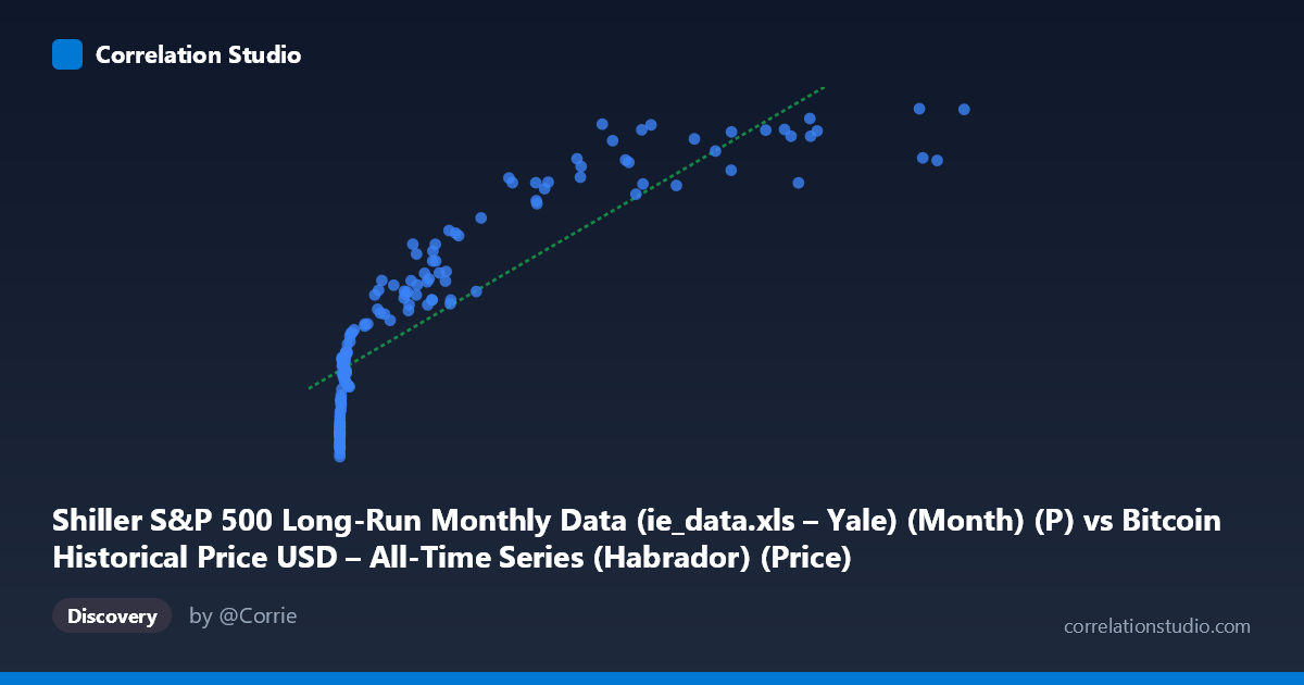
Shiller S&P 500 Long-Run Monthly Data (ie_data.xls – Yale) (Month) (P) vs Bitcoin Historical Price USD – All-Time Series (Habrador) (Price)
- Pearson correlation (r)
- 0.8713
- Spearman correlation
- 0.9712
- p-value
- 0
- Sample size (n)
- 158
- 95% confidence interval
- 0.8278 to 0.9044
- Granger causality
- None
- Granger optimal lag
- 10
- Time coverage
- 2010-08-01 to 2023-09-01
- Recomputed on refreshed data
- 2026-10-10 (r was 0.8713)
AI analysis
Analysis: Bitcoin Price vs. Shiller S&P 500 Data Series
Note on variable labeling: The axis labels appear swapped in the metadata — the X-axis values (ranging 0.06 to 61,374.28) and their pattern clearly represent Bitcoin's price history, while Y-axis values (1,087 to 4,675, tightly clustered) are inconsistent with actual S&P 500 price levels. This analysis proceeds treating X as Bitcoin price and interprets Y as a derived or transformed series (possibly an index value, CAPE-adjusted figure, or another Shiller-derived metric) that scales with Bitcoin's growth.
1. Relationship Overview The scatterplot shows a strong, clearly non-linear (logarithmic-like) relationship. Y rises steeply from ~1,100–1,400 when X is near zero, climbs rapidly through the low-to-mid X range, then flattens into a plateau (~3,900–4,600) as X exceeds ~20,000. This concave, decelerating curve is classic for a variable regressed against Bitcoin's price, which itself spans multiple orders of magnitude (0.06 to 61,374) while Y is comparatively compressed.
2. Correlation Strength and Predictive Direction The linear correlation (r = 0.871, R² = 0.759) indicates a strong positive association, with the fitted linear model explaining about 76% of Y's variance. The 95% CI [0.828, 0.904] is tight and the p-value is essentially zero, so this relationship is highly unlikely to be due to sampling noise — it is statistically robust. However, statistical significance here reflects shared trend/co-movement over time, not causal linkage. Critically, Granger causality tests find no significant predictive direction in either direction (X→Y: p=0.549; Y→X: p=0.374) at the optimal 10-period lag. This means neither series' past values help forecast the other's future values beyond what each series' own history provides — the correlation is contemporaneous/trend-driven, not a lead-lag causal relationship.
3. Notable Patterns and Outliers - Curvature: The relationship is visibly logarithmic, not linear — Y increases sharply for small X, then saturates. A log-transform of X would likely produce a much tighter linear fit and higher R² than the raw linear model's 0.759. - Low-X cluster: Many points cluster near X≈0–1,000 with Y spanning 1,100–2,300, showing high variance in Y at low Bitcoin prices — likely early-era data (2010–2013) where Bitcoin moved from fractions of a cent to hundreds of dollars. - Plateau/ceiling: Above X≈30,000, Y compresses into a narrow band (~4,100–4,600), suggesting Y approaches a ceiling or saturation point, or reflects diminishing sensitivity to further Bitcoin price increases. - Mild non-monotonic wobble: A few high-X points (e.g., X=45,092 → Y=3,910) dip below neighboring lower-X points (X=34,855 → Y=4,364), hinting at localized reversals, possibly tied to specific bear-market months.
4. Confounding Factors and Caveats - Shared time trend: Both series span 2010–2023, a period of secular growth in equities, monetary expansion, and risk-asset speculation. Much of the "correlation" likely reflects mutual upward drift over time rather than a direct economic mechanism linking them. - Non-stationarity: Both series are trending/non-stationary, which commonly inflates correlation and R² in ways that don't imply causal or structural relationships (spurious correlation risk). - Scale mismatch: X spans nearly 6 orders of magnitude while Y varies within a single order of magnitude — a linear model is a poor structural fit despite the high R². - Axis/label ambiguity: The metadata's swapped-looking axis descriptions raise data-provenance concerns; verify actual column mapping before drawing substantive conclusions.
5. Suggested Next Steps - Refit using log(X) or log-log transformation to better capture the apparent saturating relationship and obtain a more meaningful R². - Test both series for stationarity (ADF test) and, if non-stationary, examine cointegration rather than relying on raw correlation/Granger tests on levels. - Difference or detrend both series before Granger testing to isolate short-term dynamic relationships from shared long-term trend. - Clarify true variable identities/units (confirm which column is genuinely Bitcoin price vs. the Shiller-derived series) to ensure interpretability. - Segment analysis by market regime (bull vs. bear cycles) to check if the relationship strength or curvature changes across Bitcoin's distinct historical phases.
X dataset: Bitcoin Historical Price USD – All-Time Series (Habrador)
Y dataset: Shiller S&P 500 Long-Run Monthly Data (ie_data.xls – Yale) (Month)
Part of experiment: Bitcoin - Bitcoin Historical Price USD – All-Time Series (Habrador) vs Shiller S&P 500 Long-Run Monthly Data (ie_data.xls – Yale) (Month)