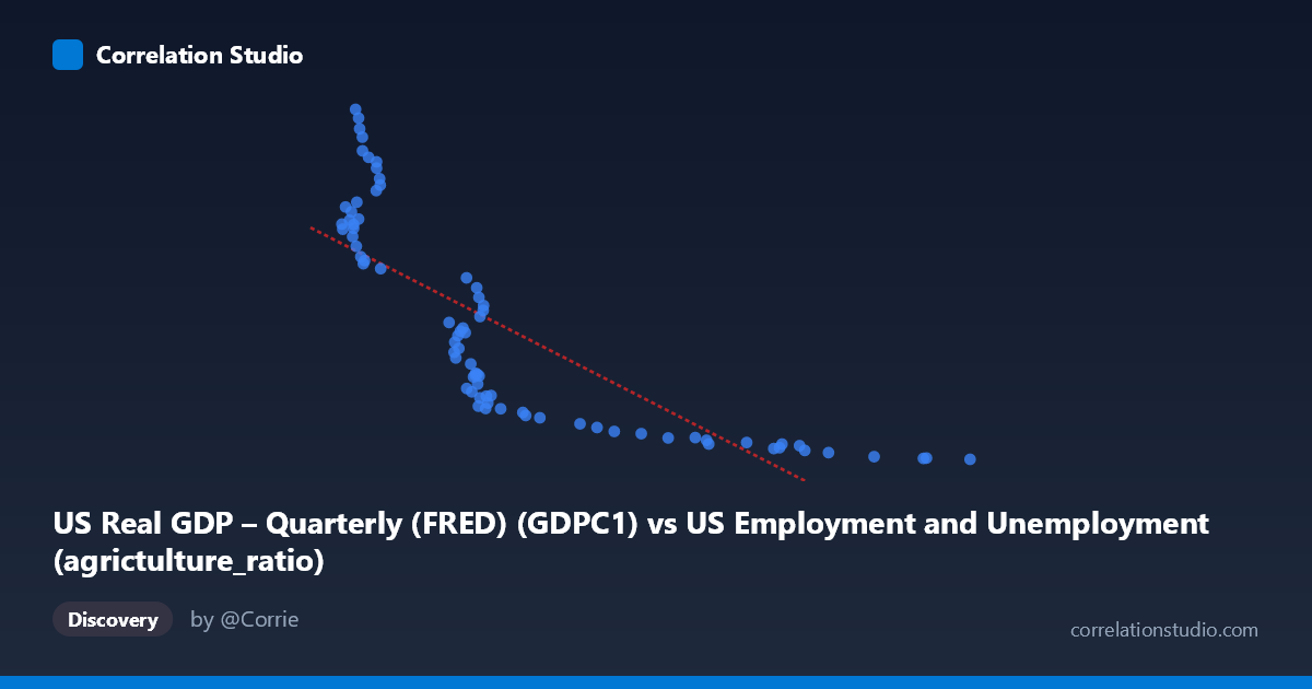
US Real GDP – Quarterly (FRED) (GDPC1) vs US Employment and Unemployment (agrictulture_ratio)
- Pearson correlation (r)
- -0.8
- Spearman correlation
- -0.924
- p-value
- 0
- Sample size (n)
- 79
- 95% confidence interval
- -0.8676 to -0.7033
- Granger causality
- None
- Granger optimal lag
- 10
AI analysis
Analysis of US Real GDP vs. Agricultural Employment Ratio
1. What the Visualization Reveals
The scatterplot displays a strong negative relationship between US Real GDP (quarterly, in billions of chained 2017 dollars) and the agricultural employment ratio in the United States, spanning data from 1947 to 2025. As GDP rises, the share of employment in agriculture falls markedly — a classic structural transformation pattern well-documented in development economics. The data points trace a curved, sweeping arc rather than a straight line, with the bulk of observations clustering in two broad zones: a lower-GDP, high-agriculture-ratio region (roughly GDP < 3,500, agriculture ratio 8,000) and a higher-GDP, low-agriculture-ratio region (GDP 5,000, agriculture ratio < 4,000). This visual shape immediately signals that the underlying relationship is likely hyperbolic or logarithmic rather than strictly linear.
2. Correlation Strength, Direction, and Temporal Predictability
The Pearson correlation of r = −0.80 confirms a strong negative association, and the R² = 0.64 tells us that approximately 64% of the variance in the agricultural employment ratio is statistically explained by the level of real GDP. This is a meaningful explanatory share, though it also means 36% of the variance remains unexplained by GDP alone — attributable to other structural, technological, and policy forces. The 95% confidence interval of [−0.87, −0.70] is tight and entirely negative, reinforcing that this inverse relationship is not a statistical artifact. The p-value ≈ 0 leaves essentially no doubt about statistical significance at any conventional threshold. However, the Granger causality tests reveal no significant predictive directionality in either direction (X→Y: F = 1.38, p = 0.22; Y→X: F = 1.53, p = 0.16), meaning that — at least at the tested lag of 10 periods — changes in GDP do not statistically precede changes in the agricultural ratio, nor vice versa. This is a critical caveat: the correlation is real, but it reflects a shared long-run trend (likely driven by common underlying forces like technological progress and industrialization) rather than a straightforward causal chain in either direction.
3. Notable Patterns, Clusters, and Non-Linearity
The most striking visual feature is the non-linearity of the scatter. The Spearman ρ exceeding Pearson r directly corroborates this: a logarithmic or power-law curve would fit substantially better than the fitted linear regression line (y = −3.30x + 22,318.7). At low GDP levels (2,095–3,500 range), the agricultural ratio spans an enormous range — from roughly 5,300 to 23,548 — suggesting high variability during the early postwar decades when agricultural transition was most dynamic. At higher GDP values (above 5,500), the agricultural ratio compresses tightly near the floor (2,182–3,500), indicating that once agricultural employment share falls below a threshold, further GDP growth yields diminishing further declines. Several high-leverage outliers appear at the upper-left of the chart — points like (2,225; 23,548), (2,254; 23,082), (2,264; 22,440), and (2,290; 21,933) — representing early postwar years when agriculture still employed a substantial fraction of the workforce. These points have disproportionate influence on the regression slope and deserve careful treatment in any modeling exercise.
4. Confounding Factors and Interpretive Caveats
Several important confounds complicate a straightforward causal interpretation. First, both variables are strongly trended over time — GDP grows secularly while agricultural employment share declines secularly — meaning much of this correlation may simply reflect shared temporal trends rather than a direct economic mechanism. The failure of Granger causality tests supports this interpretation. Second, the mechanization of agriculture, rural-to-urban migration, trade liberalization, and government farm policy all independently drive agricultural employment ratios, yet none of these appear in the model. Third, dataset alignment deserves scrutiny: GDP is quarterly (FRED GDPC1) while the employment data appears to be annual from BLS, introducing temporal aggregation mismatch that could distort the correlation. Fourth, the note that Spearman ρ Pearson r means the linear R² of 0.64 likely understates the true monotonic relationship strength — a non-linear model would explain more variance. Finally, the confidence interval and p-value assume independence of observations, which is violated here given obvious autocorrelation in both time series.
5. Actionable Insights and Further Investigation
Given the clear non-linearity, the most immediate modeling improvement would be to fit a logarithmic or inverse regression (e.g., Y = a / X^b or Y = a − b·ln(X)), which would likely improve R² substantially beyond 0.64. Researchers should also consider first-differencing or detrending both series to isolate cyclical co-movement from shared long-run trends before drawing any causal conclusions. A vector error correction model (VECM) testing for cointegration would be more appropriate than Granger causality in levels for two potentially cointegrated I(1) series. It would also be valuable to decompose the agricultural employment ratio by farm type, region, or technology adoption era to identify structural break points — the post-1970 Green Revolution and post-1990 globalization periods likely exhibit distinct dynamics. Finally, controlling for total factor productivity in agriculture and capital intensity would help disentangle whether GDP growth drives agricultural labor displacement or whether agricultural productivity gains free up labor that enables GDP growth — a distinction with significant policy implications for developing economies undergoing similar structural transitions today.
X dataset: US Employment and Unemployment
Y dataset: US Real GDP – Quarterly (FRED)
Part of experiment: Yearly - US Employment and Unemployment vs US Real GDP – Quarterly (FRED)