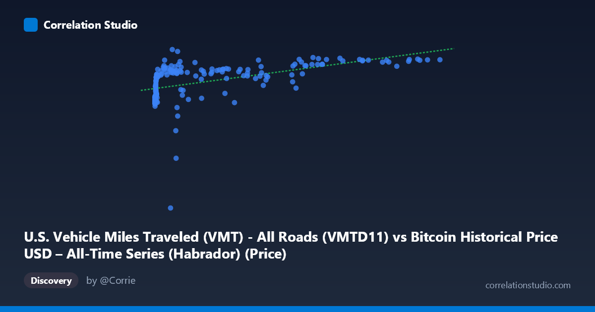
U.S. Vehicle Miles Traveled (VMT) - All Roads (VMTD11) vs Bitcoin Historical Price USD – All-Time Series (Habrador) (Price)
- Pearson correlation (r)
- 0.4939
- Spearman correlation
- 0.7421
- p-value
- 0
- Sample size (n)
- 187
- 95% confidence interval
- 0.3772 to 0.5952
- Granger causality
- None
- Granger optimal lag
- 10
AI analysis
Analysis: Bitcoin Price vs. U.S. Vehicle Miles Traveled
1. What the Visualization Reveals
This scatterplot pairs Bitcoin's historical USD price against U.S. Vehicle Miles Traveled (VMT), two series that are conceptually unrelated but happen to share a time axis (2010–2026). The plot shows a rising, concave pattern: as Bitcoin's price (X) increases from near-zero into the tens of thousands, VMT (Y) climbs from roughly 245,000 to nearly 280,000 million miles, but the relationship flattens at higher X values rather than continuing linearly. Most data points cluster at low Bitcoin prices (under $2,000) where VMT still varies substantially (245,000–270,000), indicating that early Bitcoin price movements coincide with a wide range of VMT outcomes — a sign that the relationship is weak and likely driven by shared time trends rather than direct interaction.
2. Strength, Direction, and Statistical Uncertainty
The Pearson correlation (r = 0.494) indicates a moderate positive association, but r² = 0.244 shows that only about 24% of the variance in VMT is explained by Bitcoin price — leaving roughly 76% unexplained by this relationship alone. The 95% CI [0.377, 0.595] is reasonably tight and excludes zero, and the extremely small p-value (6.8e-13) confirms the correlation is statistically significant and not due to chance, even with a moderate sample size (n=187). However, statistical significance here should not be conflated with practical or causal importance — the effect size is modest. Critically, the Granger causality tests show no significant predictive direction in either direction (X→Y: p=0.646; Y→X: p=0.473), meaning neither series helps forecast the other's future values. This strongly suggests the correlation is spurious or mediated by a third factor (most likely the shared upward trend over calendar time), rather than reflecting any real causal or leading/lagging relationship.
3. Notable Patterns and Non-linear Features
The data shows a clear non-linear, logarithmic-like shape: VMT rises steeply as Bitcoin price moves from near-zero to a few thousand dollars, then plateaus even as Bitcoin price extends into the tens of thousands (e.g., points near X=97,000–118,000 cluster around Y=276,000–278,000, similar to points at X=57,000–62,000). This flattening explains why Spearman's rank correlation would exceed Pearson's — the relationship is monotonic but not linear. One notable outlier is (8,640, 224,870), where VMT drops well below the surrounding trend, likely corresponding to a real-world VMT disruption (e.g., pandemic-related travel decline) independent of Bitcoin price. The extreme right-skew in X (Bitcoin's exponential price growth) also compresses most observations into the low end of the X-axis, exaggerating the appearance of a strong pattern at a glance.
4. Confounding Factors and Caveats
The most important caveat is that both variables are independently trending upward over the 2010–2026 window — Bitcoin due to speculative adoption/growth cycles, and VMT due to population growth, economic recovery, and post-pandemic travel rebound. This shared time trend is a classic confounder that can produce moderate correlation between two unrelated series (a well-known "spurious correlation via co-trending" problem). The VMT dip around 2020 (COVID-19) coincides with a period of relatively low Bitcoin prices, which may be artificially inflating the correlation, while post-2020 recovery in both series adds to it. Since Granger causality found no predictive relationship, this reinforces that the correlation is very likely non-causal and driven by their common trajectory over time rather than genuine interaction between crypto markets and driving behavior.
5. Actionable Insights and Further Investigation
Given the lack of Granger causality and modest r², this correlation should not be used for forecasting one variable from the other. To test the "common trend" hypothesis, analysts should detrend both series (e.g., using year-over-year differences or removing a fitted time trend) and re-examine the correlation on residuals — if it disappears, this confirms the relationship is spurious. Additionally, fitting a logarithmic model (Y ~ log(X)) is worth exploring given the concave shape and the Spearman/Pearson discrepancy noted. Finally, researchers should treat this pairing primarily as a cautionary example of coincidental correlation between unrelated economic/behavioral time series, rather than pursue policy or investment implications from it.
X dataset: Bitcoin Historical Price USD – All-Time Series (Habrador)
Y dataset: U.S. Vehicle Miles Traveled (VMT) - All Roads
Part of experiment: Bitcoin - Bitcoin Historical Price USD – All-Time Series (Habrador) vs U.S. Vehicle Miles Traveled (VMT) - All Roads