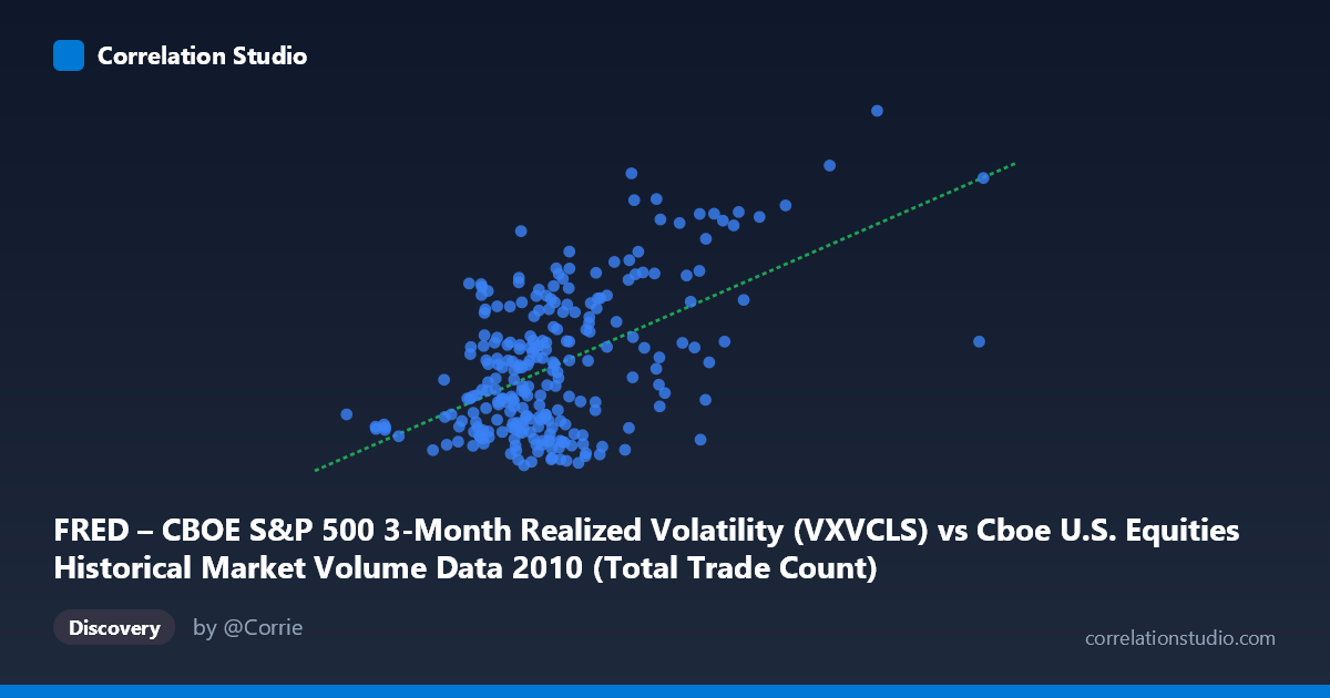
FRED – CBOE S&P 500 3-Month Realized Volatility (VXVCLS) vs Cboe U.S. Equities Historical Market Volume Data 2010 (Total Trade Count)
- Pearson correlation (r)
- 0.5328
- Spearman correlation
- 0.3713
- p-value
- 0
- Sample size (n)
- 252
- 95% confidence interval
- 0.4381 to 0.6159
- Granger causality
- Y → X
- Granger optimal lag
- 1
AI analysis
Analysis: CBOE S&P 500 3-Month Realized Volatility vs. U.S. Equities Total Trade Count (2010)
Relationship Overview
The scatterplot reveals a moderate positive relationship between CBOE S&P 500 3-Month Realized Volatility (VXVCLS) and U.S. Equities Total Trade Count across 252 trading days in 2010. As volatility increases, trade counts tend to rise as well — a pattern consistent with well-established market microstructure theory, where elevated uncertainty drives greater trading activity. The linear regression equation (y = 3.597×10⁻⁶x + 16.82) suggests that for every one-unit increase in trade count (X), realized volatility rises by approximately 3.6 millionths of a unit, though the practical framing is better read in the reverse direction given the Granger causality findings discussed below.
Correlation Strength and Statistical Significance
The Pearson correlation of r = 0.533 indicates a moderate positive association, but the explanatory power is notably limited: R² = 0.284 means only ~28.4% of the variance in realized volatility is explained by trade count, leaving over 71% attributable to other factors. The 95% confidence interval for r [0.438, 0.616] is reasonably tight and does not approach zero, and the p-value of effectively 0 (against N = 3,302 underlying observations) confirms this relationship is highly unlikely to be a statistical artifact. That said, statistical significance with large N can be somewhat misleading — the modest R² is the more honest indicator of practical predictive strength here. The Granger causality analysis adds an important directional nuance: Y Granger-causes X (F = 8.10, p = 0.0048) at a 1-period lag, meaning past values of realized volatility have statistically significant predictive power over subsequent trade counts, while the reverse direction (X→Y: F = 3.47, p = 0.064) falls just short of conventional significance thresholds. This suggests the temporal arrow points from volatility spikes to subsequent surges in trading activity, not the other way around.
Patterns, Clusters, and Outliers
The scatterplot exhibits notable heteroscedasticity — the spread of volatility values widens considerably at higher trade counts, indicating the relationship becomes less predictable in high-volume regimes. Several visible clusters are worth noting: a dense cluster of points at lower trade counts (roughly X < 2.5M) with volatility spanning a wide range (approximately 19–31), and a sparser but influential cluster at higher trade counts (X 3M) that tends to anchor the upper-right region of the chart. A few clear outliers are apparent, most notably the point near (5,514,534; 36.62) — an extreme trade count observation paired with elevated volatility — and several high-volatility points (36) at moderate trade counts around 2.8–3.6M, which suggest episodes where volatility was high independently of volume surges. These outliers may disproportionately influence the regression slope and correlation estimate.
Confounding Factors and Caveats
Several important caveats apply. First, the axis labeling appears transposed relative to the dataset descriptions — the "X" column label references VXVCLS (volatility) while the dataset it draws from is the market volume data, and vice versa for Y; analysts should verify the mapping before drawing firm conclusions. Second, 2010 was a distinctive market year, encompassing the May 6 Flash Crash and its aftermath, which likely drives some of the high-volatility, high-volume observations and may not generalize to other periods. Third, realized volatility is a backward-looking, smoothed measure (3-month window), which creates inherent lag relative to daily trade count fluctuations — this structural mismatch can both inflate and deflate apparent correlations depending on the market regime. Finally, macroeconomic announcements, earnings seasons, and index rebalancing events are common drivers of both variables simultaneously, making this correlation susceptible to omitted variable bias.
Actionable Insights and Further Investigation
Given that volatility Granger-causes trade count at a 1-day lag, traders and market structure analysts could explore whether realized volatility spikes provide short-term predictive signals for next-day volume regimes — potentially useful for execution scheduling, liquidity provisioning, or market-making strategy calibration. Further investigation should include: (1) regime-segmented analysis separating pre- and post-Flash Crash periods to test structural stability; (2) incorporating implied volatility (VIX) alongside realized volatility to disentangle forward-looking fear from backward-looking turbulence; (3) testing non-linear models (e.g., piecewise regression or quantile regression) given the visible heteroscedasticity; and (4) controlling for day-of-week and macro announcement effects to isolate the volatility-volume channel more cleanly. The moderate R² strongly suggests a richer multivariate model is warranted before any predictive application.
X dataset: Cboe U.S. Equities Historical Market Volume Data 2010
Y dataset: FRED – CBOE S&P 500 3-Month Realized Volatility
Part of experiment: Daily - Cboe U.S. Equities Historical Market Volume Data 2010 vs FRED – CBOE S&P 500 3-Month Realized Volatility