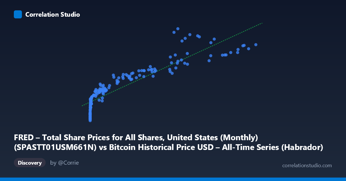
FRED – Total Share Prices for All Shares, United States (Monthly) (SPASTT01USM661N) vs Bitcoin Historical Price USD – All-Time Series (Habrador) (Price)

Pearson correlation (r): 0.9026
Spearman correlation: 0.9768
p-value: 0
Sample size (n): 189
95% confidence interval: 0.8723 to 0.9261
Granger causality: None
Granger optimal lag: 1

AI analysis

Analysis: Bitcoin Price vs. US Total Share Price Index

1. Relationship Overview

The scatterplot reveals a strong, positive, but distinctly non-linear (logarithmic-style) relationship between Bitcoin's historical price (X-axis) and the US Total Share Price Index (Y-axis). Given that X spans nearly six orders of magnitude (from $0.06 to $118,670), while Y varies only modestly (roughly 65–218), the data exhibits a classic curve typical of pairing a rapidly compounding asset against a comparatively stable macro index. Most of the visual "spread" and steepest Y-axis movement occurs at very low X-values, while at high Bitcoin prices, the curve appears to flatten as it approaches the linear fit.

2. Strength, Direction, and Statistical Confidence

The correlation coefficient (r = 0.90) indicates a strong positive linear association, with r² = 0.815 meaning approximately 81.5% of the variance in the share price index is statistically "explained" by Bitcoin's price under this linear model. The 95% confidence interval [0.872, 0.926] is tight and does not cross zero, and the p-value of ~0 confirms this correlation is highly unlikely to be due to chance. However, statistical significance and practical causality are different things: the Granger causality tests show no significant predictive direction in either direction (X→Y: p=0.474; Y→X: p=0.191). This is a critical caveat — it strongly suggests the correlation is not driven by one variable temporally leading or forecasting the other, but rather reflects a shared underlying trend (e.g., both assets rising over the same historical period due to independent macro forces like time, liquidity expansion, or risk appetite).

3. Notable Patterns and Outliers

Several features stand out: - Compressed low-end cluster: Dozens of points with X < 1000 crowd tightly near Y = 65–110, reflecting Bitcoin's early years (2010–2013) when its price was negligible while equities traded in a normal historical range. - Curved trajectory: The point cloud bends — rising steeply in Y for small increases in X early on, then flattening as X grows into the tens of thousands. This is a strong signature that a log-transform of X (or log-log model) would fit far better than the current linear model. - Late-stage divergence: At the highest X-values (e.g., X≈68,074, Y=213.35 vs. X≈86,473, Y=205.57), Y increases become erratic relative to X, suggesting increased noise/volatility in the index-BTC relationship at Bitcoin's peak valuations — possibly reflecting different macro regimes (e.g., 2021 bull run vs. 2024-2025 conditions).

4. Confounding Factors and Caveats

The most significant confound is shared time trend: both series have generally risen over 2010–2026, so much of the correlation may be spurious, driven by co-trending rather than any genuine economic linkage. Neither variable is stationary, which is a classic problem for time-series correlation and can inflate r and r² substantially. Additionally, this is a "N vs n" mismatch (833 population points reduced to 189 paired samples) — suggesting substantial data alignment/interpolation was needed, possibly introducing sampling artifacts. The Granger non-causality result further supports treating this as coincidental co-trending rather than a mechanistic relationship.

5. Suggestions for Further Investigation

- Detrend and test stationarity: Apply first-differencing or percentage-change transformations to both series and re-run correlation/Granger tests to see if the relationship holds after removing the shared trend — it likely will weaken substantially. - Log-log transformation: Given the extreme skew in X, a log(X) vs Y (or log-log) regression would likely yield a better-fitting and more interpretable model than the current linear one. - Control for common macro drivers: Introduce third variables (e.g., Fed funds rate, M2 money supply, inflation) as covariates to test whether both series are jointly responding to liquidity/monetary conditions rather than each other. - Segment by regime: Analyze correlation separately across BTC bull/bear cycles (2011-13, 2017-18, 2020-21, 2022-24) to check whether the relationship is stable or regime-dependent.

X dataset: Bitcoin Historical Price USD – All-Time Series (Habrador)

Y dataset: FRED – Total Share Prices for All Shares, United States (Monthly)

Part of experiment: Bitcoin - Bitcoin Historical Price USD – All-Time Series (Habrador) vs FRED – Total Share Prices for All Shares, United States (Monthly)