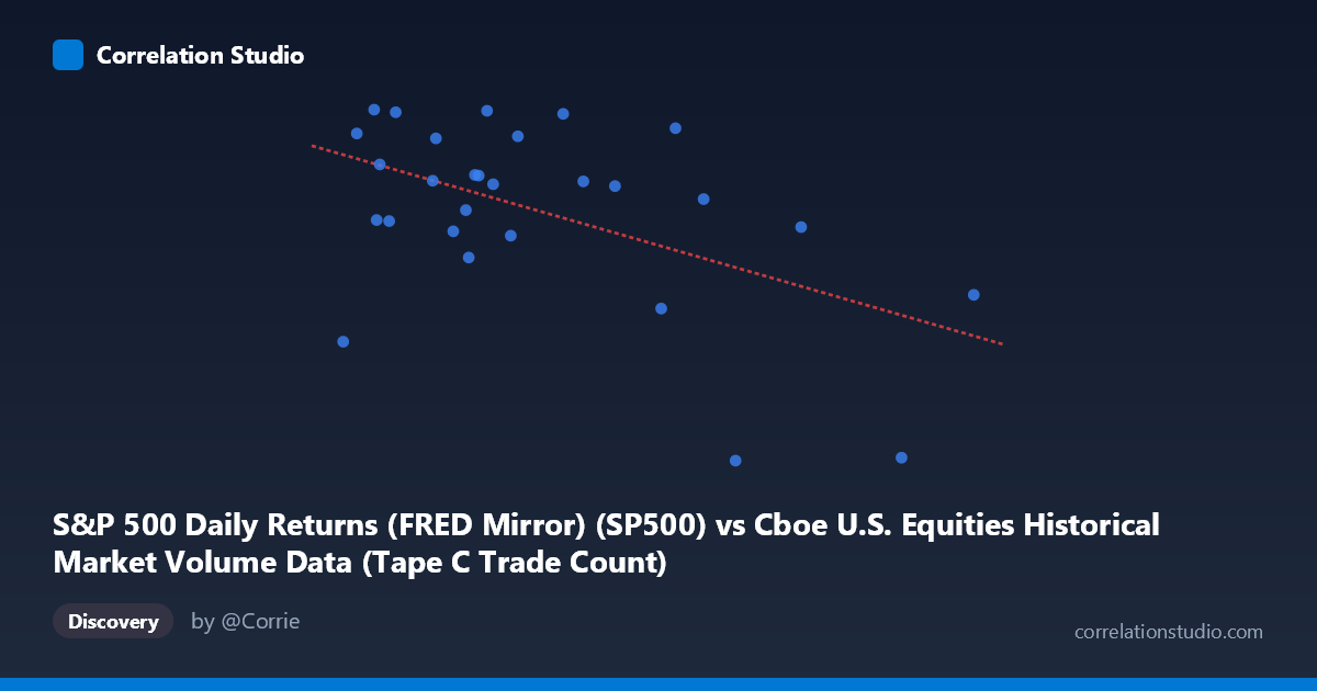
S&P 500 Daily Returns (FRED Mirror) (SP500) vs Cboe U.S. Equities Historical Market Volume Data (Tape C Trade Count)
- Pearson correlation (r)
- -0.5147
- Spearman correlation
- -0.3317
- p-value
- 0.005069
- Sample size (n)
- 28
- 95% confidence interval
- -0.7448 to -0.1753
- Granger causality
- None
- Granger optimal lag
- 7
AI analysis
Analysis: S&P 500 Daily Returns vs. Cboe Tape C Trade Count
Relationship Overview The scatterplot reveals a moderate negative relationship between S&P 500 daily price levels (X-axis, drawn from the FRED mirror) and Cboe U.S. Equities Tape C trade counts (Y-axis). As the S&P 500 index value increases, Tape C trade counts tend to decline, following the linear regression equation y = -6.00353E-05x + 7122.11. This inverse pattern is visually apparent across the data range, though with considerable scatter around the regression line, indicating the relationship is real but far from deterministic. The downward slope is subtle in absolute terms — spanning roughly 181 basis points on the Y-axis across the full X range — yet statistically meaningful given the sample characteristics.
Correlation Strength and Statistical Significance The Pearson correlation of r = -0.5147 indicates a moderate negative association, but the more practically informative metric is r² = 0.2649, meaning only about 26.5% of variance in Tape C trade counts is explained by S&P 500 price levels. The remaining ~73.5% of variation is attributable to other factors entirely. The 95% confidence interval of [-0.7448, -0.1753] is notably wide, reflecting the modest sample size of n = 28 paired observations drawn from a population of N = 1,980 — this interval does not cross zero, lending credibility to the negative direction, but the breadth signals genuine uncertainty about the true magnitude. The p-value of 0.005069 clears the conventional α = 0.05 threshold comfortably, confirming the correlation is statistically significant and unlikely to be a chance artifact. Critically, however, Granger causality tests reveal no significant temporal predictive direction in either direction (X→Y: F = 2.34, p = 0.160; Y→X: F = 3.24, p = 0.087) at the optimal 7-period lag. This means that while a contemporaneous correlation exists, neither variable reliably predicts the other's future values — the relationship should not be interpreted as causal or actionable for forecasting in its current form.
Notable Patterns, Clusters, and Outliers Several features stand out on the scatterplot. The bulk of observations cluster in the X range of approximately 2,850,000 to 3,400,000, where Tape C trade counts are relatively elevated and tightly grouped between roughly 6,900 and 6,978 — suggesting a zone of relatively stable, high trading activity at moderate index levels. Two points at the far right of the distribution (~4,162,722 and ~4,341,729) and one at ~3,751,452 correspond to notably lower trade counts (6,798, 6,883, and 6,797 respectively), anchoring the negative slope and exerting disproportionate leverage on the regression. The point at (3,751,452, 6,796.86) appears to be the most extreme low on the Y-axis and warrants particular scrutiny as a potential outlier. On the left tail, (2,779,111, 6,858.47) is also somewhat anomalous — lower trade count despite a lower index value, deviating from the general trend. These high-leverage points at the distribution extremes may be inflating the observed correlation.
Confounding Factors and Caveats Several important caveats temper interpretation. First, the dataset metadata appears to contain a labeling inconsistency — the X-axis is described as "S&P 500 Daily Returns" yet the values (2.7M–4.3M range) are clearly index price levels, not returns, which are typically expressed as percentages or small decimals. This suggests a potential data pipeline or labeling error that should be investigated before drawing conclusions. Second, the time window is narrow (January 2–February 11, 2026, approximately 41 trading days), capturing a single market regime that may not generalize. Third, omitted variables almost certainly drive much of the relationship — market volatility (VIX), macroeconomic announcements, options expiration cycles, and algorithmic trading patterns all influence Tape C trade counts independently of index levels. Fourth, the n = 28 sample drawn from 1,980 observations means ~98.6% of the population is unsampled, increasing the risk that the observed pattern reflects sampling bias rather than a robust structural relationship.
Actionable Insights and Further Investigation Given the statistically significant but modest correlation and absent Granger causality, practitioners should avoid using S&P 500 price levels alone as a predictor of Tape C trading activity. Immediate priorities should include: (1) auditing the data labeling to confirm whether X represents price levels or true daily returns, as this fundamentally changes the interpretive framework; (2) expanding the sample to utilize all 1,980 available observations to improve statistical power and reduce confidence interval width; (3) incorporating volatility measures (e.g., VIX, realized volatility) as covariates, since high-volatility episodes are known to drive trade fragmentation across tapes independently of price direction; and (4) testing non-linear specifications (e.g., quadratic or regime-switching models), as the cluster structure visible in the mid-range and the outlier behavior at extremes suggest the relationship may not be uniformly linear. A rolling-window correlation analysis across the full 2009–present dataset available in the Cboe historical files would also help determine whether this negative relationship is structurally persistent or a transient artifact of the early 2026 market environment.
X dataset: Cboe U.S. Equities Historical Market Volume Data
Y dataset: S&P 500 Daily Returns (FRED Mirror)
Part of experiment: Daily - Cboe U.S. Equities Historical Market Volume Data vs S&P 500 Daily Returns (FRED Mirror)