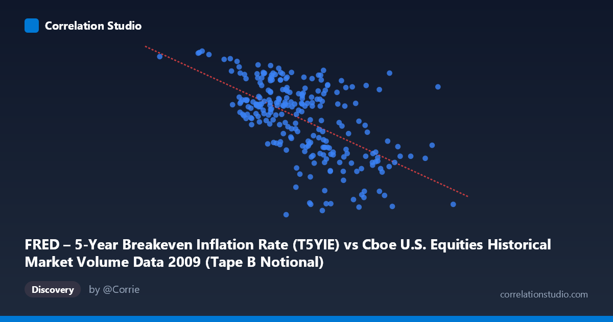
FRED – 5-Year Breakeven Inflation Rate (T5YIE) vs Cboe U.S. Equities Historical Market Volume Data 2009 (Tape B Notional)
- Pearson correlation (r)
- -0.5836
- Spearman correlation
- -0.5538
- p-value
- 0
- Sample size (n)
- 250
- 95% confidence interval
- -0.6599 to -0.4954
- Granger causality
- None
- Granger optimal lag
- 1
AI analysis
Analysis: 5-Year Breakeven Inflation Rate vs. Cboe Tape B Notional Volume (2009)
Relationship Overview
The scatterplot reveals a moderate negative relationship between Cboe U.S. Equities Tape B notional trading volume and the 5-year breakeven inflation rate during 2009. The linear regression equation (y = -2.427×10⁻¹⁰x + 2.422) indicates that as notional trading volume increases, the inflation breakeven rate tends to decline. This inverse pattern is visually coherent with the 2009 macro context: early in the year, extreme market stress and volatility drove enormous trading volumes while simultaneously suppressing inflation expectations to near-zero or negative territory, whereas as markets stabilized through mid-to-late 2009, volumes normalized downward and inflation expectations recovered toward historically typical levels near 2%.
Correlation Strength and Statistical Significance
The Pearson correlation of r = -0.584 represents a moderate negative association, with r² = 0.341 indicating that roughly 34% of the variance in breakeven inflation rates is statistically explained by variation in Tape B notional volume. While this is a meaningful share, it equally underscores that 66% of the variance remains unexplained by this single variable alone. The 95% confidence interval of [-0.660, -0.495] is reasonably tight and does not cross zero, and the p-value of effectively 0 confirms the correlation is highly unlikely to be a chance artifact given n=250 paired observations from a population of N=3,232. However, the Granger causality results tell a critical story: neither direction of temporal predictability reaches significance (X→Y: F=0.021, p=0.885; Y→X: F=1.714, p=0.192). This means that despite the robust contemporaneous correlation, neither variable meaningfully predicts the future values of the other — a vital caveat against any causal interpretation.
Notable Patterns and Outliers
Several structural features stand out in the sampled data. There is a visible cluster of high-volume, low-inflation observations (X 7×10⁹, Y < 0.6) consistent with the crisis-peak trading environment of early 2009, when inflation expectations briefly turned negative or near-deflationary. Conversely, observations with lower volumes (X < 4×10⁹) predominantly show breakeven rates above 1.5–2.1, reflecting the recovery phase. A few notable outliers exist: the point near (1.32×10⁹, 2.05) sits at an extreme low volume with elevated inflation expectations, and (2.43×10⁹, 2.11) follows similarly, possibly corresponding to late 2009 trading days with lighter volumes as conditions normalized. The relationship also appears to exhibit some non-linear compression at higher volume levels, where Y values cluster near zero with relatively little spread, suggesting a potential floor effect on inflation expectations during stress periods.
Confounding Factors and Interpretive Caveats
The most significant caveat is that both variables are jointly driven by the 2009 financial crisis trajectory — a classic case of spurious correlation through shared common cause. The Federal Reserve's unprecedented interventions, the recovery from the March 2009 market bottom, and the broader credit crisis unwinding simultaneously influenced both equity trading volumes and inflation expectations. The axes in the provided data appear to be swapped in labeling (X contains the inflation rate values per the data description, but the column names suggest a reversal), which warrants verification before drawing firm conclusions. Additionally, Tape B specifically covers NYSE American and regional exchanges, which may not fully represent broader market volume dynamics. The dataset covers only a single calendar year, limiting generalizability.
Actionable Insights and Further Investigation
Given the compelling but potentially spurious correlation, the most productive next steps would include: (1) controlling for a crisis/recovery regime variable (e.g., VIX levels or NBER recession indicators) to test whether the correlation persists within regimes; (2) expanding the time series beyond 2009 to determine if the relationship holds across different macroeconomic environments or is unique to crisis conditions; (3) testing total consolidated equity volume rather than Tape B alone to assess robustness; and (4) incorporating intermediate variables such as credit spreads or Fed balance sheet size that likely mediate both series. The absence of Granger causality strongly suggests this relationship is best interpreted as a coincident indicator of macro regime, not a predictive trading signal — any model treating volume as a forecaster of inflation expectations (or vice versa) in real-time would likely fail out-of-sample.
X dataset: Cboe U.S. Equities Historical Market Volume Data 2009
Y dataset: FRED – 5-Year Breakeven Inflation Rate
Part of experiment: Daily - Cboe U.S. Equities Historical Market Volume Data 2009 vs FRED – 5-Year Breakeven Inflation Rate