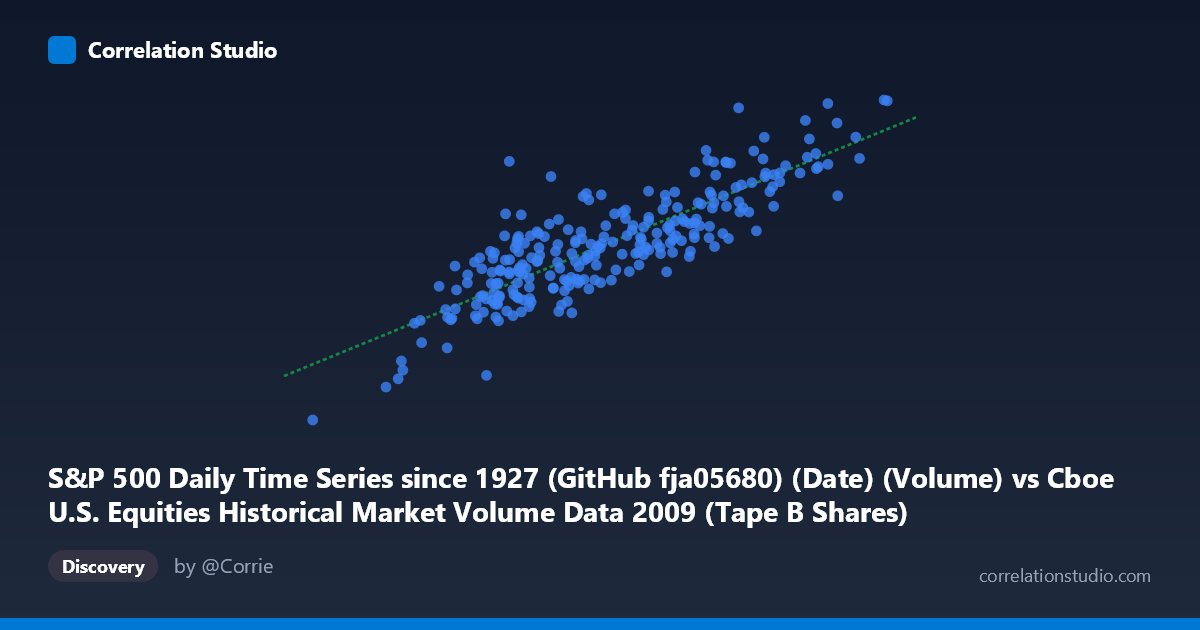
S&P 500 Daily Time Series since 1927 (GitHub fja05680) (Date) (Volume) vs Cboe U.S. Equities Historical Market Volume Data 2009 (Tape B Shares)
- Pearson correlation (r)
- 0.8448
- Spearman correlation
- 0.8237
- p-value
- 0
- Sample size (n)
- 252
- 95% confidence interval
- 0.8053 to 0.8769
- Granger causality
- None
- Granger optimal lag
- 10
AI analysis
Scatterplot Analysis: S&P 500 Daily Volume vs. Cboe Tape B Shares (2009)
Relationship Overview The scatterplot reveals a strong positive linear relationship between S&P 500 daily trading volume (X-axis) and Cboe Tape B share volume (Y-axis) across 252 trading days in 2009. As total market volume increases, Tape B share volume rises in a broadly consistent, upward-sloping pattern. The linear regression equation (y = 25.9952x + 1.756×10⁹) suggests that for every additional unit of total market volume, Tape B shares increase by approximately 26 units, with a substantial baseline intercept reflecting Tape B's persistent share of activity even at lower volume levels. The data spans a meaningful range — total volume from ~34M to ~256M and Tape B shares from ~1.27B to ~9.12B — capturing the full spectrum of 2009 market conditions, including the volatile post-financial-crisis recovery period.
Correlation Strength and Statistical Significance The Pearson correlation of r = 0.8448 indicates a strong positive association, and the R² of 0.7138 means that approximately 71.4% of the variance in Tape B share volume is explained by total market volume — a substantial but incomplete explanatory share. The remaining ~28.6% is attributable to other factors not captured here. The 95% confidence interval of [0.8053, 0.8769] is relatively narrow, reflecting reliable estimation precision given the sample of n = 252 paired observations drawn from a population of N = 3,232. The p-value of effectively 0 confirms the correlation is highly statistically significant and extremely unlikely to be a chance finding. However, Granger causality tests reveal no significant predictive temporal direction in either direction (X→Y: F = 0.655, p = 0.765; Y→X: F = 1.437, p = 0.166), meaning that while the two series move together contemporaneously, neither reliably leads or predicts the other across the optimal 10-period lag. This is a critical distinction: the correlation is real, but it appears to be concurrent co-movement rather than a causal or predictive relationship.
Notable Patterns, Clusters, and Outliers The data exhibits a reasonably tight central cluster between roughly 100M–200M total volume and 4B–7.5B Tape B shares, consistent with typical 2009 trading days. However, several notable features stand out. At the upper extreme, a point near (254M, 9.12B) sits slightly above the regression line, likely corresponding to a high-volatility session during early 2009 market stress. At the lower extreme, the point at approximately (34M, 1.27B) is a clear outlier — likely a holiday-shortened session or anomalous low-volume day — and its leverage on the regression line warrants scrutiny. There also appears to be modest heteroscedasticity: the spread around the regression line widens at higher volume levels, suggesting that the relationship becomes less predictable during peak-activity sessions. A handful of points in the mid-range (e.g., ~115M X but ~6.3B Y) sit noticeably above the fitted line, hinting at days where Tape B attracted disproportionate activity relative to total market volume.
Confounding Factors and Caveats Several important caveats apply. First, both variables are volume-based metrics measured on the same underlying market, so the strong correlation may partly reflect definitional overlap — Tape B shares are a component of the broader market volume ecosystem, meaning they are not fully independent series. This could artificially inflate the observed correlation. Second, 2009 was an extraordinary year — spanning the tail of the financial crisis, the March 2009 market bottom, and the subsequent recovery rally — meaning volatility regimes shifted substantially intra-year. The relationship may not be stable across sub-periods. Third, trading venue fragmentation (the rise of alternative trading systems and dark pools in 2009) could independently drive both metrics upward, acting as a common latent driver. Fourth, the absence of Granger causality at a 10-period lag does not rule out same-day or instantaneous co-movement driven by shared exogenous shocks, which the contemporaneous correlation likely captures.
Actionable Insights and Further Investigation Despite the absence of Granger causality, the strong R² of 71.4% makes total market volume a useful proxy or control variable for modeling Tape B activity, particularly in risk management or liquidity estimation contexts. Practitioners could explore whether the unexplained ~28.6% variance correlates with specific market events (FOMC announcements, earnings seasons, index rebalancing days), which would add explanatory power. Sub-period analysis — splitting 2009 into the crisis phase (Jan–March) and recovery phase (April–December) — could reveal whether the regression slope or intercept shifts materially across regimes. It would also be valuable to test shorter lag structures (1–3 days) for Granger causality, as the 10-period optimal lag may obscure shorter-term predictive signals. Finally, examining the outlier at (34M, 1.27B) specifically — confirming whether it represents a legitimate trading day or a data anomaly — is advisable before using this regression for forecasting purposes.
X dataset: Cboe U.S. Equities Historical Market Volume Data 2009
Y dataset: S&P 500 Daily Time Series since 1927 (GitHub fja05680) (Date)
Part of experiment: Daily - Cboe U.S. Equities Historical Market Volume Data 2009 vs S&P 500 Daily Time Series since 1927 (GitHub fja05680) (Date)