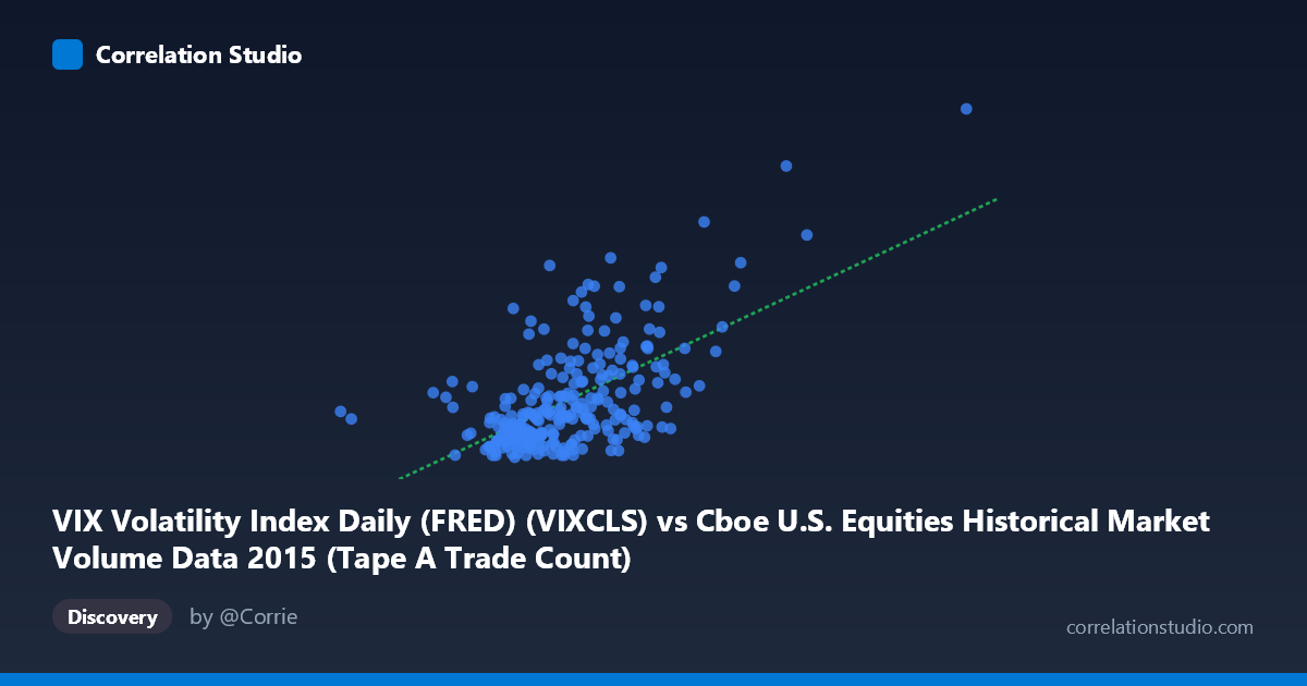
VIX Volatility Index Daily (FRED) (VIXCLS) vs Cboe U.S. Equities Historical Market Volume Data 2015 (Tape A Trade Count)
- Pearson correlation (r)
- 0.6064
- Spearman correlation
- 0.5158
- p-value
- 0
- Sample size (n)
- 252
- 95% confidence interval
- 0.522 to 0.6791
- Granger causality
- None
- Granger optimal lag
- 1
AI analysis
Analysis: VIX Volatility Index vs. Tape A Trade Count (2015)
Relationship Overview The scatterplot reveals a moderate positive relationship between the VIX Volatility Index and Cboe Tape A Trade Count across 252 trading days in 2015. As implied volatility rises, equity trade counts on Tape A tend to increase — a directionally intuitive finding, since elevated market fear and uncertainty characteristically drive higher trading activity as investors rebalance, hedge, or exit positions. The linear regression equation (y = 1.03×10⁻⁵x + 1.921) confirms this upward slope, though the relatively shallow gradient suggests that large increases in trade volume correspond to meaningful but not dramatic swings in VIX.
Correlation Strength and Statistical Framing The Pearson correlation of r = 0.606 indicates a moderate positive association, but the explanatory power is more sobering: R² = 0.368, meaning VIX explains roughly 36.8% of the variance in Tape A trade counts, leaving nearly two-thirds of variation attributable to other factors. The 95% confidence interval [0.522, 0.679] is reasonably tight and sits entirely above zero, reinforcing genuine signal rather than noise. The p-value of ~0 confirms high statistical significance given n = 252. However, the Granger causality results are notably absent of significance — neither X→Y (F = 0.244, p = 0.622) nor Y→X (F = 0.212, p = 0.646) reaches conventional thresholds at lag-1. This is a critical caveat: while the contemporaneous correlation is real, VIX does not temporally predict trade counts (or vice versa) one period ahead, suggesting the relationship is largely coincident rather than directionally causal.
Notable Patterns, Clusters, and Outliers The data exhibits a clear clustering of observations in the lower-left quadrant — the majority of days feature VIX readings between roughly 1.0M–1.6M (notional X units) and trade counts below 20, reflecting relatively calm 2015 market conditions for much of the year. However, several prominent high-leverage outliers are visible in the upper-right region, including points near (2,247,816; 36.02) and (2,076,907; 28.03), which correspond to periods of acute volatility — likely the August 2015 China-driven market selloff. One anomalous low-X outlier at approximately (576,208; 15.74) warrants attention, as it departs substantially from the X-axis range and may reflect a data anomaly, holiday-shortened session, or exchange disruption. The spread around the regression line also widens at higher VIX values, suggesting heteroscedasticity — the relationship is less predictable under stressed conditions.
Confounding Factors and Caveats Several confounds complicate causal interpretation. Secular intraday and day-of-week patterns in trade volume are independent of VIX but could inflate apparent correlation. Market microstructure changes in 2015, including algorithmic trading surges during volatility spikes, may drive both variables simultaneously without a true causal link. The fact that Tape A specifically captures NYSE-listed securities means the measure is not comprehensive of total market activity, introducing selection bias. Additionally, the dataset covers only one calendar year — a period that included an unusual volatility regime shift in August — making the correlation potentially unrepresentative of other market environments. The Granger non-causality result also warns against any forward-looking trading strategy based solely on this relationship.
Actionable Insights and Further Investigation Practitioners should avoid interpreting VIX as a leading indicator of Tape A volume given the failed Granger tests; any trading or risk management rule based on this lag structure would lack empirical grounding. More productive avenues include: (1) testing longer lag structures (2–5 periods) in Granger causality to detect slower transmission effects; (2) decomposing trade count into buyer-initiated vs. seller-initiated flows to assess whether VIX spikes asymmetrically drive selling pressure; (3) extending the analysis across multiple years to test whether the 2015 August shock unduly dominates the correlation estimate; and (4) introducing control variables such as S&P 500 returns, bid-ask spreads, or options volume to isolate VIX's incremental explanatory contribution. A non-linear or regime-switching model may also better capture the apparent heteroscedasticity at high-volatility extremes.
X dataset: Cboe U.S. Equities Historical Market Volume Data 2015
Y dataset: VIX Volatility Index Daily (FRED)
Part of experiment: Daily - Cboe U.S. Equities Historical Market Volume Data 2015 vs VIX Volatility Index Daily (FRED)