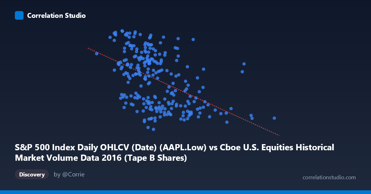
S&P 500 Index Daily OHLCV (Date) (AAPL.Low) vs Cboe U.S. Equities Historical Market Volume Data 2016 (Tape B Shares)
- Pearson correlation (r)
- -0.4773
- Spearman correlation
- -0.4919
- p-value
- 0
- Sample size (n)
- 252
- 95% confidence interval
- -0.5674 to -0.3759
- Granger causality
- None
- Granger optimal lag
- 1
AI analysis
Scatterplot Analysis: AAPL Low Price vs. Cboe Tape B Share Volume (2016)
Relationship Overview The scatterplot reveals a negative relationship between Apple's daily low price (X-axis) and Cboe Tape B share volume (Y-axis) across 252 trading days in 2016. As AAPL's low price increases, Tape B share volume tends to decline. The linear regression equation (y = -1.21115E⁻⁰⁷x + 116.67) quantifies this inverse trend, with the negative slope confirming that higher AAPL prices are associated with lower Tape B volumes. The data cloud is moderately dispersed, suggesting the relationship is real but far from deterministic, with considerable day-to-day variability around the trend line.
Correlation Strength and Statistical Significance The Pearson correlation of r = -0.4773 indicates a moderate negative association. However, the coefficient of determination (r² = 0.2279) is the more practically meaningful figure — it tells us that only 22.8% of the variance in Tape B share volume is explained by AAPL's low price, leaving roughly 77% attributable to other factors. The 95% confidence interval of [-0.5674, -0.3759] is entirely negative, confirming directional consistency, and the p-value of 8.88×10⁻¹⁶ is extraordinarily small, making it essentially certain this correlation did not arise by chance in the sample. That said, statistical significance here is partly a function of the large sample (n = 252), and practical significance remains modest. Critically, the Granger causality tests show no significant predictive directionality in either direction (X→Y: F = 1.35, p = 0.246; Y→X: F = 0.62, p = 0.432), meaning that past values of AAPL's low price do not meaningfully forecast next-period Tape B volume, and vice versa. The correlation is contemporaneous, not predictive.
Notable Patterns, Clusters, and Outliers The sample points reveal a broad scatter across the AAPL low price range of roughly $89–$117, with the bulk of observations clustering between $90–$115 and X values between ~75M–130M. A few notable features stand out: points at the lower end of AAPL prices (near $89–$93) appear predominantly at higher X values (larger share volumes), consistent with the negative trend. Conversely, several high-Y observations (e.g., ~116–117) appear at relatively low X values (~75M–80M). There are potential outliers on the high-X end — one point near X = 170M with Y ≈ 94.9 stands out as an unusually high-volume day — which may exert leverage on the regression line. No strong non-linear curvature is immediately apparent, but the wide vertical spread at mid-range X values suggests heteroscedasticity or latent subgroups within the data.
Confounding Factors and Interpretive Caveats This correlation almost certainly reflects shared macroeconomic or market-wide dynamics rather than a direct causal mechanism between AAPL's price floor and Tape B volumes. In 2016, AAPL experienced a notable price trough in the first half of the year followed by recovery — a period that also coincided with shifting overall equity market volumes. Tape B shares (primarily NYSE American/regional exchange listings) respond to broad market sentiment, liquidity cycles, and regulatory/structural factors largely independent of AAPL's valuation. The dataset mismatch — X comes from an S&P 500 OHLCV dataset while Y comes from Cboe market structure data — raises the question of whether a confounding third variable (e.g., VIX, overall market turnover, or macroeconomic events like Brexit in June 2016) drives both series simultaneously. The absence of Granger causality reinforces that any apparent relationship is likely spurious or coincidental in a temporal sense.
Actionable Insights and Further Investigation Given that 77% of Tape B volume variance remains unexplained, multivariate modeling incorporating broader market indicators (overall S&P 500 level, VIX, Fed policy dates, earnings announcements) would substantially improve explanatory power. Researchers should test whether the negative correlation persists when controlling for market-wide volume trends — if it disappears, the relationship is likely a statistical artifact of shared time trends rather than a meaningful signal. Segmenting the data by market regime (e.g., pre- vs. post-Brexit, Q1 selloff vs. Q4 rally) could reveal whether the correlation is stable or driven by a specific sub-period. Finally, given the Granger null result, this variable pair should not be used for short-term forecasting in either direction; any trading or operational strategy relying on this relationship as a predictive signal would lack empirical support.
X dataset: Cboe U.S. Equities Historical Market Volume Data 2016
Y dataset: S&P 500 Index Daily OHLCV (Date)
Part of experiment: Daily - Cboe U.S. Equities Historical Market Volume Data 2016 vs S&P 500 Index Daily OHLCV (Date)