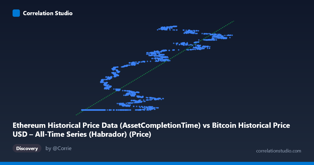
Ethereum Historical Price Data (AssetCompletionTime) vs Bitcoin Historical Price USD – All-Time Series (Habrador) (Price)
- Pearson correlation (r)
- 0.8726
- Spearman correlation
- 0.9398
- p-value
- 0
- Sample size (n)
- 3926
- 95% confidence interval
- 0.865 to 0.8799
- Granger causality
- None
- Granger optimal lag
- 10
AI analysis
Analysis: Ethereum "Completion Time" vs. Bitcoin Historical Price
Note on labeling: The axis labels appear swapped or mismatched in the metadata—X is described as an "AssetCompletionTime" column from a Bitcoin dataset, while Y is described as "Price" from an Ethereum dataset. Given the actual values (X ranges ~209 to ~124,720; Y ranges ~$1.6B to ~$1.78B), this looks like X is likely an ETH price-like series (or index) and Y is a large cumulative/timestamp-like or market-cap-like figure rather than a simple spot price. The analysis below treats the data at face value as two positively associated numeric series, but the labeling should be verified before drawing asset-specific conclusions.
1. Relationship Revealed by the Visualization The scatterplot shows a strong, positive, and notably non-linear relationship. A large cluster of points sits at low X values (roughly 200–20,000) where Y is nearly flat at ~1,614,335,000 — suggesting a floor or saturation effect at low X. Above X ≈ 20,000, Y begins rising steadily and near-linearly, climbing to ~1.78B as X approaches 125,000. This pattern resembles a threshold/step relationship followed by a linear regime rather than a pure straight-line correlation across the whole range.
2. Strength, Direction, and Statistical Confidence The Pearson correlation (r = 0.8726) indicates a strong positive linear association, with r² = 0.7615 meaning about 76% of the variance in Y is statistically explained by X in a linear model — a substantial but not complete explanatory power, leaving ~24% of variance driven by other factors or non-linear dynamics. The 95% CI [0.8650, 0.8799] is tight, and the p-value is effectively 0, confirming the correlation is highly unlikely to be due to chance given the large sample (n=3,926). However, correlation strength does not imply causation: the Granger causality tests show no significant predictive direction in either direction (X→Y: p=0.96; Y→X: p=0.72), meaning neither series' past values help forecast the other's future values at any tested lag. This strongly suggests the relationship is contemporaneous/structural (e.g., both driven by a shared underlying trend like time or market cycles) rather than one variable temporally leading the other.
3. Notable Patterns and Features - Flat-then-rising shape: The dominant visual feature is a "hockey stick" — Y is pinned near its minimum (~1.614B) for a wide swath of low-to-mid X values, then increases roughly linearly once X exceeds ~20,000–40,000. - Clustering: A dense cluster of points exists at very low X (under 12,000) all mapping to nearly identical Y values, suggesting these may represent an early/stable period (e.g., early market history before price discovery or before Ethereum's launch). - Linear regime at high X: For X 40,000, points align closely with the fitted regression line (slope ≈ 1,402 per unit X), suggesting a more classic linear relationship once outside the "floor" zone. - No obvious outliers: Points seem to follow one of the two regimes without erratic scatter, though the two-regime shape violates simple linearity assumptions.
4. Confounding Factors and Caveats - Time as a lurking variable: Given this is time-series data spanning 2015–2026, both series likely trend upward over time due to shared macro factors (crypto market growth, inflation, adoption), inflating correlation without direct causal linkage — classic spurious correlation risk in trending time series. - Non-stationarity: Both variables likely have unit roots/trends; Pearson r and linear R² can be misleading for non-stationary series. Consider first-differencing or cointegration tests instead. - Label ambiguity: As noted, axis descriptions are confusing/possibly mismatched, and Y's huge scale (~1.6 billion) doesn't correspond to typical BTC or ETH spot prices — it may be a cumulative metric, timestamp, or market cap in smaller currency units. This must be clarified before drawing asset-based conclusions. - Two-regime structure: Fitting a single linear model across a floor-then-rise pattern understates the true complexity; R²=0.76 may be an artifact of the flat cluster anchoring the line rather than genuine proportional co-movement throughout.
5. Suggested Next Steps - Clarify data provenance: Confirm what X and Y actually represent (price, market cap, cumulative volume, etc.) and check units/timestamps for mismatched joins. - Segment the analysis: Split data into the "floor" regime (low X) and "linear" regime (high X) and model each separately, or use a piecewise/spline regression to better capture the hockey-stick shape. - Test for spurious trend correlation: Run correlation on de-trended or differenced series, or perform a cointegration test (e.g., Engle-Granger) given the shared time-based drift and lack of Granger causality. - Investigate the flat cluster: Determine whether the many identical low-X/low-Y points reflect a specific historical period (e.g., pre-2017 crypto markets) that may need separate treatment or exclusion. - Reconsider causal claims: Given no Granger causality in either direction, avoid claiming one asset "predicts" the other; instead frame the relationship as contemporaneous co-movement likely driven by common market-wide factors.
X dataset: Bitcoin Historical Price USD – All-Time Series (Habrador)
Y dataset: Ethereum Historical Price Data
Part of experiment: Bitcoin - Bitcoin Historical Price USD – All-Time Series (Habrador) vs Ethereum Historical Price Data