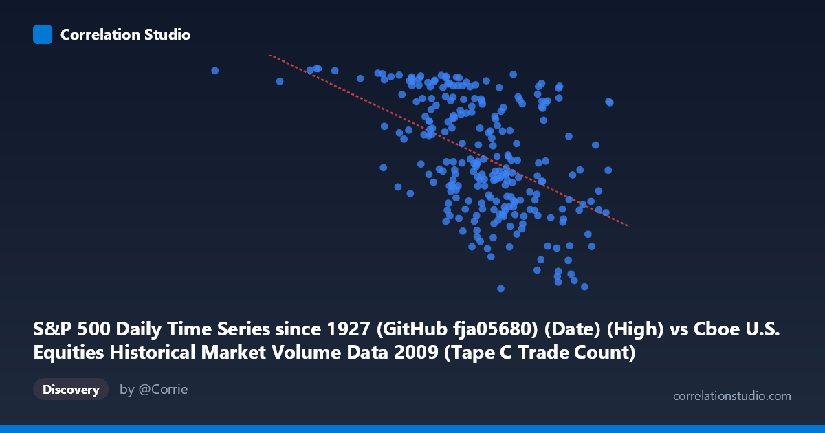
S&P 500 Daily Time Series since 1927 (GitHub fja05680) (Date) (High) vs Cboe U.S. Equities Historical Market Volume Data 2009 (Tape C Trade Count)
- Pearson correlation (r)
- -0.4994
- Spearman correlation
- -0.5026
- p-value
- 0
- Sample size (n)
- 252
- 95% confidence interval
- -0.5868 to -0.4005
- Granger causality
- None
- Granger optimal lag
- 4
AI analysis
Analysis: S&P 500 Daily High vs. Cboe Tape C Trade Count (2009)
Relationship Overview The scatterplot reveals a moderate negative relationship between the S&P 500 daily high price (X-axis) and the Cboe Tape C trade count (Y-axis) across 252 trading days in 2009. As the S&P 500 high increases — moving from the crisis lows near 185,887 toward recovery highs approaching 848,554 — trade counts on Tape C tend to decline. This pattern is consistent with the well-documented "fear-driven volume" phenomenon: elevated trading activity during market stress and panic selling in early 2009, followed by quieter, more orderly markets as prices recovered through the year. The linear regression equation (y = −0.000564x + 1,314.79) confirms this inverse trajectory.
Correlation Strength and Statistical Significance The Pearson correlation of r = −0.4994 indicates a moderate negative association, but the more informative metric is r² = 0.2494, meaning only about 25% of the variance in Tape C trade counts is explained by the S&P 500 daily high. Three-quarters of the variation remains unexplained by this single predictor alone. The 95% confidence interval of [−0.587, −0.401] is reasonably tight and entirely negative, providing strong evidence that the inverse relationship is real and not a sampling artifact. The p-value of effectively zero confirms statistical significance at any conventional threshold, which is unsurprising given the sample of n = 252 from a population of N = 3,232. However, the Granger causality results are notably inconclusive: neither X→Y (F = 2.40, p = 0.051) nor Y→X (F = 2.41, p = 0.050) reaches conventional significance at the 5% level, with both hovering tantalizingly at the boundary. This means we cannot confidently assert a temporal predictive direction — price does not robustly predict future trade counts, nor does trade count robustly predict future prices, at least at the 4-period optimal lag tested.
Notable Patterns and Outliers Several features stand out in the sample points. There is a prominent outlier at approximately (185,887; 1,126) — the lowest X value in the dataset — which corresponds to the depths of the financial crisis, where an extremely low S&P 500 high coincides with very high trade activity, consistent with panic-driven volume. A cluster of points in the X range of 540,000–700,000 shows considerable vertical spread (Y values ranging from roughly 788 to 1,119), suggesting high variance in trade counts even at similar price levels. At the upper end of X (prices above 760,000), trade counts tend to compress toward lower values (700–930 range), indicating reduced trading intensity during the late-year recovery. The relationship also appears somewhat heteroscedastic — variance in Y is wider at lower X values and narrows as X increases — suggesting the linear model may not fully capture the structure of this relationship.
Confounding Factors and Caveats Several important caveats apply. Temporal autocorrelation is almost certain in both daily price and volume series, which can inflate apparent correlations and violate independence assumptions. The negative correlation likely reflects a shared dependency on a third variable: time itself — as 2009 progressed from crisis lows to recovery highs, trade volumes naturally declined from panic peaks, making this potentially a spurious correlation driven by the crisis-to-recovery arc rather than a true causal price-volume mechanism. Additionally, Tape C specifically reflects NYSE Arca trading, so it may not represent broader market volume dynamics uniformly. The S&P 500 "High" (rather than close or volume-weighted price) is an unusual choice as an independent variable and may introduce noise. The Granger causality tests operating at a 4-period lag also only capture short-term predictive relationships and could miss longer structural dependencies.
Actionable Insights and Further Investigation The near-significant Granger results (both p ≈ 0.050) warrant replication with adjusted lag structures — testing lags from 1 to 10 periods and applying corrections for multiple comparisons could clarify whether a marginal predictive relationship exists. A partial correlation analysis controlling for calendar time (trading day number) would test whether the price-volume relationship persists after removing the shared trend driven by the 2009 recovery narrative. Investigators should also explore non-linear modeling (e.g., polynomial regression or GAMs) given the heteroscedasticity and the possibility of a regime-change around mid-year. Broadening the analysis to include Tape A and Tape B counts, VIX, and bid-ask spreads as covariates would likely substantially increase explained variance beyond the current 25% and provide a richer picture of what drives trading intensity on U.S. equity exchanges.
X dataset: Cboe U.S. Equities Historical Market Volume Data 2009
Y dataset: S&P 500 Daily Time Series since 1927 (GitHub fja05680) (Date)
Part of experiment: Daily - Cboe U.S. Equities Historical Market Volume Data 2009 vs S&P 500 Daily Time Series since 1927 (GitHub fja05680) (Date)