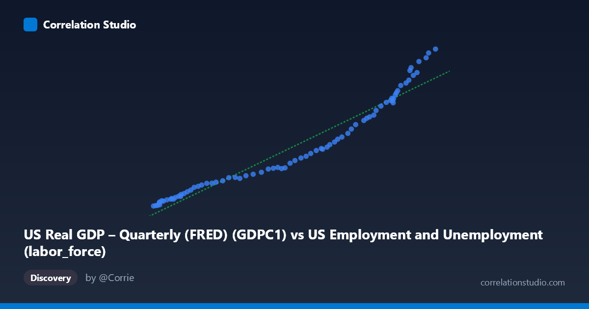
US Real GDP – Quarterly (FRED) (GDPC1) vs US Employment and Unemployment (labor_force)
- Pearson correlation (r)
- 0.9685
- Spearman correlation
- 0.9991
- p-value
- 0
- Sample size (n)
- 79
- 95% confidence interval
- 0.951 to 0.9798
- Granger causality
- None
- Granger optimal lag
- 10
- Time coverage
- 1947-01-01 to 2025-01-01
- Recomputed on refreshed data
- 2026-10-09 (r was 0.9686)
AI analysis
Analysis: US Real GDP vs. Labor Force
Relationship Overview
The scatterplot reveals a strong, positive, and largely linear relationship between US Real GDP (quarterly, in billions of chained 2017 dollars) and the US labor force (in thousands of persons). As GDP rises from roughly $60,000B to $171,000B across the observed range, the labor force grows correspondingly from approximately 2,183 to 23,548 (in the units plotted). The data points cluster tightly around the fitted regression line y = 0.1678x − 8,961.62, suggesting that over the 1947–2025 time horizon, economic output and labor force size have expanded together in a remarkably consistent long-run trajectory. This co-movement is consistent with standard macroeconomic growth theory: a larger productive population supports greater output, and a growing economy draws more workers into participation.
Correlation Strength and Statistical Significance
The correlation is exceptionally strong (r = 0.9686), and the coefficient of determination (R² = 0.9383) indicates that 93.8% of the variance in labor force size is explained by variation in real GDP within this sample. The 95% confidence interval [0.9513, 0.9799] is narrow and entirely in the upper range, confirming the estimate is precise and not a statistical artifact of small-sample noise. With a p-value reported as 0 (effectively p < 0.0001, n = 79), there is virtually no probability this correlation arose by chance. However, the Granger causality tests complicate the interpretation significantly: neither direction — GDP predicting labor force (F = 1.484, p = 0.175) nor labor force predicting GDP (F = 1.544, p = 0.153) — achieves statistical significance at conventional thresholds, even at an optimal lag of 10 periods (~2.5 years quarterly). This means that while the two series move together strongly in level, neither reliably predicts the other's future changes in a temporal sense, suggesting the relationship reflects shared secular trends rather than a clean causal mechanism in either direction.
Patterns, Clusters, and Notable Features
The scatter is notably clean across most of the range, with points dispersing slightly at the upper end (GDP $150,000B, corresponding to the post-2010 era), where a few observations appear marginally above or below the regression line — hinting at a subtle nonlinearity or structural change in the GDP–labor force relationship in recent decades. The lower-left cluster (GDP ~$60,000–$80,000B, labor force ~2,000–5,000) likely corresponds to the late 1940s through 1960s, when both the economy and the measured labor force were smaller. The upper-right points (GDP ~$160,000–$171,000B) represent recent years and show slightly more scatter, possibly reflecting post-pandemic labor market disruptions (2020–2022), where GDP and labor force participation decoupled temporarily. No extreme outliers are visible, but the spread around the regression line does appear to widen modestly at higher values — a mild heteroscedastic pattern worth investigating.
Confounding Factors and Caveats
Several important caveats apply. First, both series share a common driver: time itself. Over 78 years, population growth, productivity improvements, and technological change all trend upward simultaneously, making it nearly impossible to disentangle genuine structural linkage from spurious co-trending. The failure to establish Granger causality reinforces this concern — correlation here is largely a story of two growing series, not of one driving the other. Second, the unit mismatch and dataset crossover (GDP is quarterly in billions of chained 2017 dollars; labor force appears to be annual employment figures from BLS, resampled or matched) introduces potential aggregation artifacts. Third, labor force participation rates have varied substantially over this period (e.g., rising female participation 1960s–1990s, Baby Boomer retirement pressures post-2008), meaning the size of the labor force conflates demographic shifts with true economic responsiveness. Finally, major structural breaks — the 1970s stagflation, the 2008 financial crisis, and the 2020 COVID shock — may temporarily violate the linear assumption embedded in the regression.
Actionable Insights and Further Investigation
Given the near-perfect linear fit historically, this relationship could serve as a baseline benchmark for labor market expectations conditional on GDP forecasts — with meaningful deviations from the regression line flagging structural labor market stress or demographic transitions. To deepen the analysis, researchers should: (1) detrend both series (e.g., using HP filter or first differences) before re-running correlation and Granger tests, which would reveal whether the relationship holds beyond shared secular drift; (2) test for structural breaks (Chow test or CUSUM) around 1980, 2008, and 2020 to assess whether the GDP–labor force elasticity has shifted over time; (3) incorporate labor force participation rate rather than raw labor force size to control for demographic composition; and (4) explore nonlinear or cointegration models (e.g., Engle-Granger or Johansen cointegration tests), which are better suited to long-run relationships between non-stationary economic series than standard OLS correlation.
X dataset: US Employment and Unemployment
Y dataset: US Real GDP – Quarterly (FRED)
Part of experiment: Yearly - US Employment and Unemployment vs US Real GDP – Quarterly (FRED)