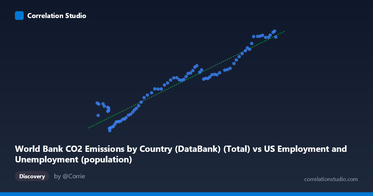
World Bank CO2 Emissions by Country (DataBank) (Total) vs US Employment and Unemployment (population)
- Pearson correlation (r)
- 0.9608
- Spearman correlation
- 0.933
- p-value
- 0
- Sample size (n)
- 80
- 95% confidence interval
- 0.9394 to 0.9748
- Granger causality
- None
- Granger optimal lag
- 10
AI analysis
Scatterplot Analysis: US Employment Population vs. World CO2 Emissions
Relationship Overview
The scatterplot reveals a strong, positive, and largely linear relationship between total world CO2 emissions and the US employment population across the period 1941–2020. As CO2 emissions rise along the x-axis (ranging from approximately 93,220 to 260,329 units), the US employment population on the y-axis climbs correspondingly from roughly 9,870 to 43,129 thousand persons. The data points track closely along the fitted regression line (y = 0.176x − 4,192), suggesting that both variables have grown in a relatively synchronized fashion over eight decades, consistent with the long-run expansion of both the global economy and the US labor force during the postwar era.
Correlation Strength and Statistical Framing
The Pearson correlation of r = 0.9608 indicates a very strong positive association, and the R² of 0.9232 means that approximately 92.3% of the variance in US employment population is statistically accounted for by variation in world CO2 emissions within this sample. The 95% confidence interval for r of [0.9394, 0.9748] is narrow and sits entirely in high-correlation territory, reinforcing that this is a robust and precisely estimated association rather than a sampling artifact. The p-value of effectively zero confirms that the correlation is highly statistically significant across the n = 80 paired observations. However, the Granger causality results tell a critically different story: neither direction of temporal prediction is statistically significant (X→Y: F = 0.749, p = 0.676; Y→X: F = 0.813, p = 0.618). At the optimal lag of 10 periods, neither variable meaningfully predicts the future values of the other once own-history is accounted for. This firmly signals that the correlation, however numerically impressive, does not reflect a directional causal or predictive mechanism between the two series.
Notable Patterns, Clusters, and Outliers
Several structural features are visible in the scatter. In the lower-left cluster (x ≈ 93,000–130,000; y ≈ 9,870–18,000), corresponding roughly to the 1940s–1960s, the points show somewhat more scatter relative to the regression line, with a few observations sitting noticeably below the fitted trend — most prominently the point near (105,000, 9,870), which likely reflects wartime or immediate postwar labor market disruption. In the mid-range (x ≈ 130,000–210,000; y ≈ 18,000–31,000), covering roughly the 1960s–1990s, points track the regression line closely with low residual spread, suggesting the most stable co-movement period. In the upper-right cluster (x ≈ 235,000–260,000; y ≈ 37,000–43,000), several points appear to plateau or compress — the y-values increase more slowly per unit of x, hinting at a possible concave non-linearity or saturation effect as both series approach their modern ceilings. This slight curvilinear tendency at the upper end is worth noting, as the linear model may marginally underfit that region.
Confounding Factors and Interpretive Caveats
The dominant confounding factor here is time itself. Both variables — global CO2 emissions and US employment population — are monotonically increasing long-run time series driven by a common underlying trend: world population growth, economic development, industrialization, and energy consumption. This is a textbook case of spurious correlation via shared secular trend; two variables that independently track global economic growth will correlate strongly with each other even if there is no direct or indirect causal link. The absence of Granger causality reinforces this interpretation. Additionally, the axis labels deserve scrutiny — the dataset metadata indicates a possible column mismatch (the x-axis is labeled as CO2 emissions but drawn from the US Employment dataset, and vice versa), which may reflect a data join artifact and warrants verification before drawing any substantive conclusions. Other confounders include post-WWII baby boom demographics, shifts in labor force participation rates (especially women entering the workforce), changes in CO2 accounting methodology over time, and structural breaks such as recessions (2008–2009) or the COVID-19 period near the end of the sample.
Actionable Insights and Further Investigation
Given that this correlation is most likely spurious and driven by shared time trends, the most important next step is detrending both series — for example, by differencing, computing year-over-year growth rates, or applying a Hodrick-Prescott filter — before drawing any interpretive conclusions. Analysts should also verify the column-to-dataset assignment flagged in the metadata, as a mislabeled join could invalidate the physical interpretation entirely. If the goal is to understand genuine links between labor markets and emissions, more theoretically motivated variables should be examined, such as emissions per employed worker, emissions intensity of GDP, or sector-specific employment in fossil fuel industries. Extending the Granger causality test to shorter, detrended subperiods (e.g., decade-by-decade windows) could reveal whether any transient predictive relationship emerges in specific economic regimes. Finally, incorporating a multivariate framework that controls for GDP, population, and energy prices would help isolate whether any residual relationship between employment and emissions survives after common macroeconomic drivers are accounted for.
X dataset: US Employment and Unemployment
Y dataset: World Bank CO2 Emissions by Country (DataBank)
Part of experiment: Yearly - US Employment and Unemployment vs World Bank CO2 Emissions by Country (DataBank)