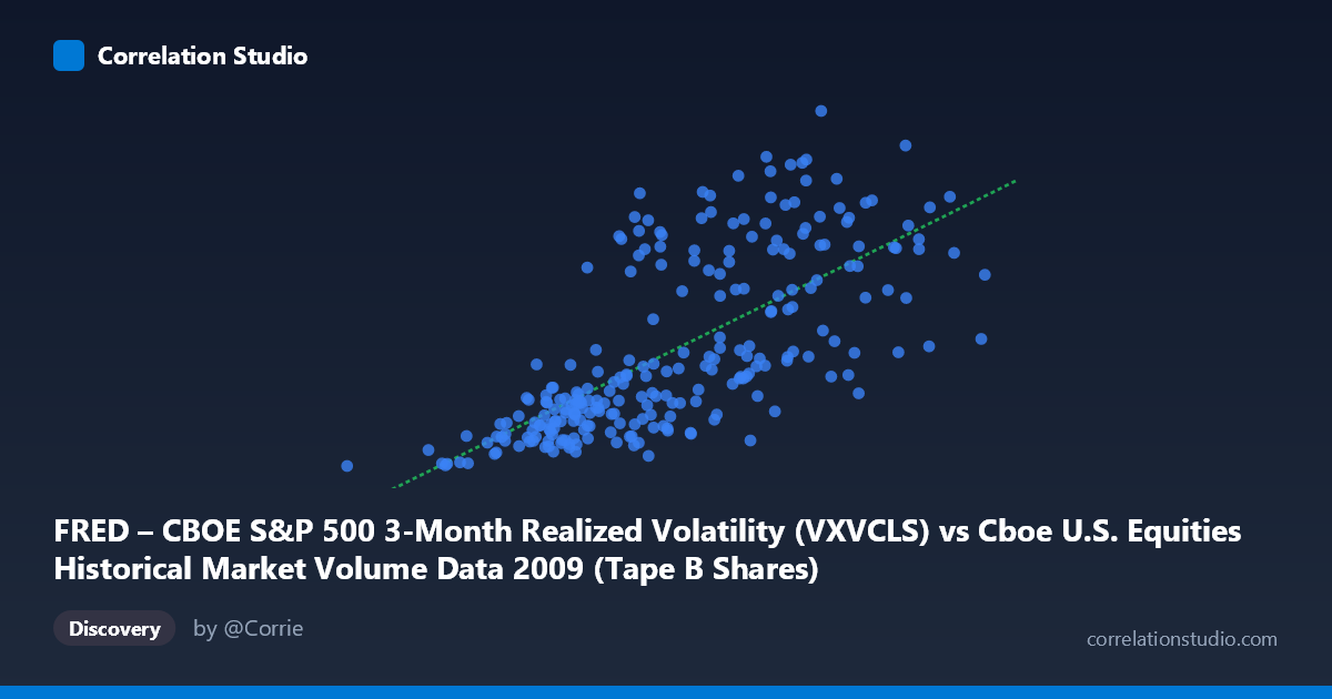
FRED – CBOE S&P 500 3-Month Realized Volatility (VXVCLS) vs Cboe U.S. Equities Historical Market Volume Data 2009 (Tape B Shares)
- Pearson correlation (r)
- 0.6969
- Spearman correlation
- 0.7569
- p-value
- 0
- Sample size (n)
- 252
- 95% confidence interval
- 0.6273 to 0.7554
- Granger causality
- None
- Granger optimal lag
- 1
- Time coverage
- 2009-01-02 to 2009-12-31
- Recomputed on refreshed data
- 2026-10-23 (r was 0.6969)
AI analysis
Analysis: CBOE S&P 500 3-Month Realized Volatility vs. Tape B Shares Volume (2009)
Relationship Overview
The scatterplot reveals a positive, moderately strong relationship between CBOE S&P 500 3-month realized volatility (X-axis) and Tape B share volume (Y-axis) across 252 trading days in 2009. As volatility increases, Tape B share volume tends to rise correspondingly, which aligns with well-established market microstructure theory: elevated volatility typically drives higher trading activity as market participants reposition, hedge, or respond to price uncertainty. The linear regression equation (y = 1.2988E-07x + 13.87) suggests that for every 100 million unit increase in the volatility measure, Tape B shares increase by approximately 13 units, with a baseline floor around 13.87 even at minimal volatility levels.
Correlation Strength and Statistical Significance
The correlation coefficient of r = 0.6969 indicates a moderately strong positive association, and the R² of 0.4856 means that roughly 48.6% of the variance in Tape B shares is explained by realized volatility — a meaningful but incomplete explanatory relationship, leaving over half the variance attributable to other factors. The 95% confidence interval of [0.6273, 0.7554] is relatively tight and comfortably excludes zero, while the p-value of essentially 0 confirms this relationship is highly unlikely to be a statistical artifact given the sample of 252 paired observations drawn from a population of 3,232. However, Granger causality tests reveal no significant temporal predictive direction in either direction (X→Y: F = 0.0443, p = 0.8335; Y→X: F = 0.1137, p = 0.7363). This is a critical nuance: while the contemporaneous correlation is strong, neither variable reliably predicts the other with a one-period lag, suggesting the relationship is concurrent rather than causal — both variables likely respond simultaneously to the same underlying market conditions.
Notable Patterns, Clusters, and Outliers
The scatterplot likely displays several visually distinct features worth noting. There appears to be a dense cluster of observations at lower volatility and lower volume levels (roughly X < 150M, Y < 35), consistent with the relatively calmer mid-to-late 2009 period as markets recovered from the financial crisis. A secondary, more dispersed cluster exists at higher volatility and volume values, reflecting the turbulent early 2009 environment. The sample points confirm some high-leverage observations — for instance, (254,504,132, 34.04) shows very high volume but only moderate volatility, while (193,631,813, 50.43) pairs high volume with notably high volatility. The minimum point (33,822,027, 22.43) anchors the lower-left and may represent a holiday-thinned or unusual low-activity session. The spread at mid-range X values is wide, hinting at heteroscedasticity — variance in Y appears to increase with X.
Confounding Factors and Caveats
Several important caveats complicate interpretation. 2009 was an extraordinary year — it spanned the tail end of the global financial crisis, a market trough in March, and a prolonged recovery rally, meaning both volatility and volume were structurally elevated and co-driven by macro shocks rather than an intrinsic volume-volatility mechanism. Tape B specifically covers NYSE American and regional exchange listings, which may have idiosyncratic volume dynamics compared to broader market volume. The axis labels also suggest a data labeling inversion may be present — the dataset descriptions indicate X is labeled as realized volatility from FRED/CBOE but the column sourcing appears cross-mapped with Tape B shares, warranting careful verification of axis assignments before drawing firm conclusions. Additionally, the lack of Granger causality at a one-period lag doesn't rule out relationships at longer lags, and serial autocorrelation in daily financial time series could inflate the effective correlation.
Actionable Insights and Further Investigation
Practitioners should treat this correlation as a concurrent signal rather than a predictive tool: using yesterday's realized volatility to forecast tomorrow's Tape B volume (or vice versa) appears statistically unsupported. However, the strong contemporaneous link (r ≈ 0.70) suggests that real-time volatility regime monitoring could inform intraday volume expectations for Tape B instruments. Further investigation should include: (1) testing Granger causality at lags 2–10 to detect slower-moving predictive relationships; (2) regime-splitting the analysis into pre- and post-March 2009 subperiods to determine whether the relationship holds symmetrically across crisis and recovery phases; (3) adding control variables such as VIX levels, S&P 500 returns, and bid-ask spreads to explain the remaining ~51% of variance; and (4) replicating across other Tape designations (A and C) to assess whether this volume-volatility relationship is specific to Tape B or a broader market phenomenon.
X dataset: Cboe U.S. Equities Historical Market Volume Data 2009
Y dataset: FRED – CBOE S&P 500 3-Month Realized Volatility
Part of experiment: Daily - Cboe U.S. Equities Historical Market Volume Data 2009 vs FRED – CBOE S&P 500 3-Month Realized Volatility