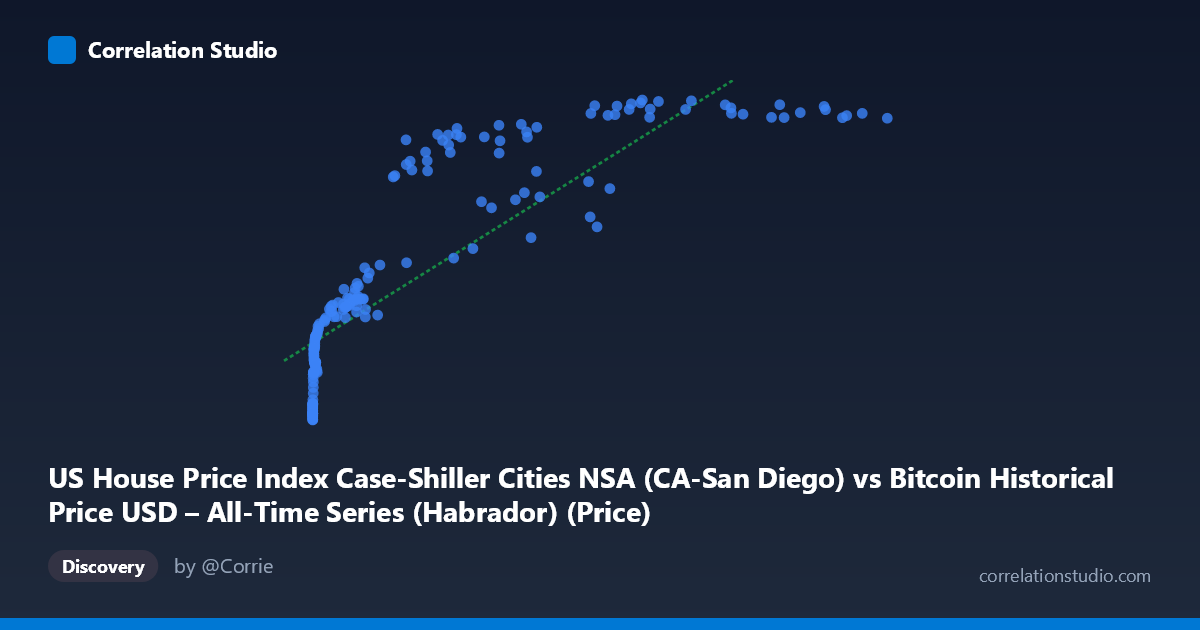
US House Price Index Case-Shiller Cities NSA (CA-San Diego) vs Bitcoin Historical Price USD – All-Time Series (Habrador) (Price)
- Pearson correlation (r)
- 0.8515
- Spearman correlation
- 0.97
- p-value
- 0
- Sample size (n)
- 191
- 95% confidence interval
- 0.8071 to 0.8863
- Granger causality
- None
- Granger optimal lag
- 9
- Time coverage
- 2010-08-01 to 2026-06-01
- Recomputed on refreshed data
- 2026-10-24 (r was 0.8469)
AI analysis
Analysis: Bitcoin Price vs. US Case-Shiller Home Price Index (San Diego)
1. What the Visualization Reveals
The scatterplot shows a strong positive association between Bitcoin's historical USD price and the Case-Shiller San Diego home price index over the 2010–2026 window. However, the shape of the relationship is distinctly non-linear: Y (home price index) rises steeply at very low X values (Bitcoin under ~$1,000), climbing from ~150 to ~250, then flattens into a long, gently-sloping plateau in the 250–450 range as X stretches out over four orders of magnitude (from hundreds to over $100,000). This is a classic logarithmic/saturating curve rather than a straight line — the data compresses heavily on the X-axis at low values and stretches at high values, which is typical when one variable (Bitcoin price) has exponential growth dynamics while the other (a home price index) grows in a much more bounded, linear/cyclical fashion.
2. Strength, Direction, and Uncertainty
The Pearson correlation (r = 0.84) is strong and positive, with r² = 0.71 indicating that a linear model explains about 71% of the variance in Y. The 95% CI [0.795, 0.880] is fairly tight and excludes zero, and the p-value is effectively 0, so the linear association is statistically robust and not a product of sampling noise. That said, the note that Spearman ρ exceeds Pearson r confirms visually what the scatter suggests: the true relationship is curved, so a log-transform of X (or a polynomial/log fit) would likely explain meaningfully more variance than the 71% captured by the naive linear model. Critically, the Granger causality tests show no significant predictive direction in either direction (X→Y: p=0.73; Y→X: p=0.82) at the optimal lag of 9 periods. This means that despite the strong contemporaneous correlation, neither series helps forecast the other's future movements — the correlation is best interpreted as two variables that have moved together (likely driven by a common macro trend) rather than one causing or leading the other.
3. Notable Patterns and Outliers
The most striking feature is the "hockey stick" shape: dozens of points cluster near the origin (X < 1,000, Y ≈ 150–230), representing Bitcoin's early years (2010–2013) when prices were negligible while home prices already sat in a moderate range. As X crosses into the thousands and tens-of-thousands, Y rises quickly then saturates around 400–450, forming a dense band at high X values (X 20,000) where Y hovers narrowly between ~300 and ~450 despite X varying by nearly 100,000 units. A few points act as local outliers relative to a smooth curve — e.g., (45,092.81, 321.37), (58,724.66, 331.59), and (56,973.18, 374.46) sit noticeably below the trend of neighboring points with similar or lower X values (e.g., 44,354 → 416), suggesting these correspond to a period where Bitcoin price dropped or home prices lagged (possibly the 2022 crypto crash / lag in housing index updates).
4. Confounding Factors and Caveats
This is a textbook case of spurious correlation via shared time trend: both Bitcoin price and the Case-Shiller index have risen substantially over 2010–2026 due to entirely different macroeconomic forces (crypto adoption/speculation vs. housing supply, interest rates, demographics). Correlating two upward-trending time series over a shared date range will almost always produce a high r even absent any causal mechanism — this is sometimes called a "nonsense regression" in econometrics. The lack of Granger causality reinforces this: there's no evidence one market leads the other. Additional caveats include the vastly different scales and variances of X (stdev 29,663 vs mean 20,037, heavily right-skewed) versus Y (stdev ~100 vs mean ~279), non-stationarity in both series (both likely have trends/unit roots, which inflates correlation and invalidates standard significance tests unless differenced), and the fact that "NSA" (not seasonally adjusted) housing data introduces cyclical/seasonal noise unrelated to Bitcoin.
5. Suggestions for Further Investigation
To get a more honest read on this relationship: (1) apply a log transform to X (and possibly Y) and refit — given Spearman Pearson, a log-linear or log-log model should substantially improve fit; (2) difference or detrend both series (e.g., use % monthly returns instead of levels) and recompute correlation and Granger tests — this is the standard fix for spurious trend-driven correlation and will likely show the "true" relationship is much weaker; (3) test for cointegration (e.g., Engle-Granger) if the goal is to argue a genuine long-run equilibrium relationship exists, rather than relying on raw-level correlation; (4) investigate the specific outlier periods (2022 Bitcoin crash points) for narrative context; and (5) consider that both series may simply be common proxies for broad monetary/liquidity conditions (e.g., Fed policy, inflation, dollar liquidity) — including a third variable like M2 money supply or real interest rates could reveal whether this is really a story about a shared macro driver rather than a direct Bitcoin–housing relationship.
X dataset: Bitcoin Historical Price USD – All-Time Series (Habrador)
Y dataset: US House Price Index Case-Shiller Cities NSA
Part of experiment: Bitcoin - Bitcoin Historical Price USD – All-Time Series (Habrador) vs US House Price Index Case-Shiller Cities NSA