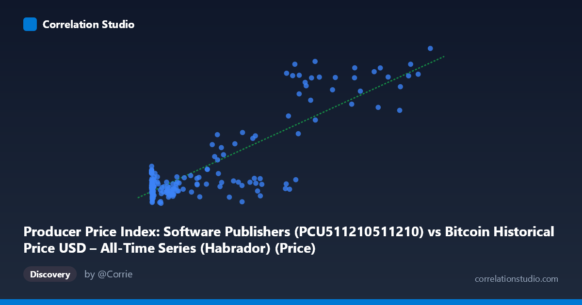
Producer Price Index: Software Publishers (PCU511210511210) vs Bitcoin Historical Price USD – All-Time Series (Habrador) (Price)
- Pearson correlation (r)
- 0.8463
- Spearman correlation
- 0.3591
- p-value
- 0
- Sample size (n)
- 189
- 95% confidence interval
- 0.8002 to 0.8824
- Granger causality
- None
- Granger optimal lag
- 1
AI analysis
Analysis: Bitcoin Price vs. Producer Price Index (Software Publishers)
1. What the Visualization Reveals
The scatterplot shows a strongly right-skewed distribution along the X-axis (Bitcoin price), with the vast majority of observations clustered below $50,000 and a sparse tail extending out to ~$118,670. The Y-axis (PPI for Software Publishers) is much more compressed, ranging narrowly from ~85 to ~103. The overall shape suggests a curve that is roughly flat-to-slightly-increasing at low X values, followed by a steep upward sweep at high Bitcoin prices — consistent with the fitted linear model but with visible curvature that a straight line only partially captures.
2. Strength, Direction, and Statistical Confidence
The correlation coefficient (r = 0.846) indicates a strong positive linear relationship, with r² = 0.716 meaning roughly 72% of the variance in the software PPI is statistically associated with Bitcoin price levels. The 95% CI [0.800, 0.882] is fairly tight and excludes zero, and the p-value of ~0 confirms this correlation is highly unlikely to be due to chance in this sample. However, the Granger causality tests tell a very different and important story: neither direction shows significant predictive power (X→Y: p=0.77; Y→X: p=0.87). This means that despite the strong contemporaneous correlation, Bitcoin price does not help forecast future PPI values, nor vice versa. In practical terms, this is a classic case of correlation without demonstrated temporal causation — both series likely trend together because of a shared external driver (e.g., time itself, inflation, or macroeconomic conditions) rather than because one leads or causes the other.
3. Notable Patterns and Outliers
The data show a clear "hockey stick" pattern: at low Bitcoin prices (under $10,000), Y values are tightly clustered between 85–89 with little variation, suggesting the PPI was essentially stable/independent of BTC price in this regime. Above roughly $50,000–60,000, Y values escalate more steeply, reaching 96–103. This suggests non-linearity — a logarithmic or power relationship may fit better than the linear model, since Bitcoin's price history spans nearly 6 orders of magnitude (from $0.06 to $118,670) while PPI only spans about 18 points. The extreme skew in X means the linear regression is heavily influenced by the handful of high-price points (e.g., the $85K–$118K cluster), which could be leverage points disproportionately driving the fit.
4. Confounding Factors and Caveats
This relationship is almost certainly spurious or indirect. Both Bitcoin price and the Software Publishers PPI have exhibited long-term upward trends over the 2010–2026 window, largely independent of one another — Bitcoin driven by adoption/speculation cycles, and the PPI driven by software industry pricing/inflation dynamics. Any two time series with a persistent trend will show high correlation without genuine causal linkage (a well-known "spurious correlation via co-trending" problem). The lack of Granger causality reinforces this: there's no evidence of a functional or economic mechanism linking BTC prices to software pricing indices. Additionally, using n=189 paired points from a population of 342 raises questions about how the sample was selected and whether monthly aggregation, interpolation, or date-matching introduces further artifacts.
5. Suggested Next Steps
Given the non-stationary, trending nature of both series, analysts should difference the data (e.g., month-over-month % changes) before computing correlation, and re-run Granger tests on the differenced series to check for genuine short-term dynamic relationships. A log-transform of Bitcoin price would also likely improve linear fit and reduce leverage effects from extreme values. Most importantly, this correlation should not be used for predictive or trading purposes — it likely reflects two unrelated series co-trending over calendar time rather than an economically meaningful link. Investigating a common third factor (e.g., overall CPI, USD strength, or time itself as a proxy) would help clarify why both metrics rise together.
X dataset: Bitcoin Historical Price USD – All-Time Series (Habrador)
Y dataset: Producer Price Index: Software Publishers
Part of experiment: Bitcoin - Bitcoin Historical Price USD – All-Time Series (Habrador) vs Producer Price Index: Software Publishers