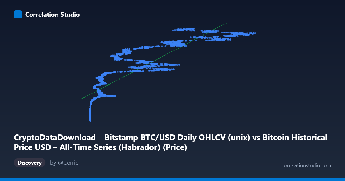
CryptoDataDownload – Bitstamp BTC/USD Daily OHLCV (unix) vs Bitcoin Historical Price USD – All-Time Series (Habrador) (Price)
- Pearson correlation (r)
- 0.847
- Spearman correlation
- 0.9491
- p-value
- 0
- Sample size (n)
- 4170
- 95% confidence interval
- 0.8382 to 0.8554
- Granger causality
- None
- Granger optimal lag
- 10
- Time coverage
- 2014-11-28 to 2026-04-28
- Recomputed on refreshed data
- 2026-10-08 (r was 0.847)
AI analysis
Analysis: Bitcoin Price (Habrador) vs. Bitstamp BTC/USD Price
1. What the Visualization Reveals
This scatterplot is actually comparing two different historical price series for the same asset (Bitcoin), sourced from different providers — one general historical dataset (Habrador) plotted against Bitstamp's daily OHLCV close price, with timestamps on the Y-axis. Given that both series track BTC/USD price over overlapping time periods, this is fundamentally a cross-source validation check rather than a study of two independent economic variables. The scatter shows a strong monotonic relationship: as the X-axis price value increases, the corresponding Unix timestamp (Y-axis) also increases — meaning higher Bitcoin prices are associated with later dates, which simply reflects Bitcoin's long-term secular price appreciation from 2014 to 2026.
2. Strength, Direction, and Statistical Confidence
The correlation is strong and positive (r = 0.847, r² = 0.7175), meaning roughly 72% of the variance in the timestamp variable is statistically explained by the price value. The 95% CI [0.838, 0.855] is tight given the large sample (n=4,170), and p ≈ 0 confirms this relationship is not due to chance. However, r² of 0.72 also means 28% of variance is unexplained — consistent with Bitcoin's well-known volatility, where price does not increase smoothly with time but moves in sharp bull/bear cycles. Critically, the Granger causality tests show no significant predictive direction in either direction (X→Y: p=0.11; Y→X: p=0.32). This confirms that neither series "temporally leads" the other — reinforcing that this is not a causal economic relationship, but rather two measurements of essentially the same underlying phenomenon (BTC price over time), where any lead/lag structure is negligible at the tested lag of 10 periods.
3. Notable Patterns and Non-linear Features
The data clearly shows clustering by market cycle: a dense cloud of low values (sub-$1,000–$10,000) spanning 2014–2020, then sparser, higher-value clusters ($20,000–$100,000+) concentrated in 2020–2026, reflecting Bitcoin's exponential-style growth punctuated by crashes. Sample points show non-monotonic reversals (e.g., $54,458 in early 2021 followed by $48,907 later, then $28,168 in 2023) indicative of boom-bust cycles rather than steady linear growth. The note that Spearman ρ exceeds Pearson r strongly suggests the true relationship is monotonic but curved (e.g., logarithmic or power-law), which is expected since Bitcoin price growth is often modeled as log-linear over time — a straight line in log(price) vs. time, not raw price vs. time.
4. Confounders and Caveats
The most important caveat: these two variables are not independent phenomena — they are two overlapping/redundant measurements of Bitcoin price (possibly from different exchanges or aggregation methods), so "correlation" here largely reflects data consistency rather than a meaningful economic relationship. Any divergence between the two (residual 28% unexplained variance) may stem from exchange-specific pricing differences (Bitstamp vs. broader market), timestamp misalignment, missing data, or genuine arbitrage spreads across venues. Additionally, using a linear model on exponential-growth financial data is a known misspecification — it will systematically underfit early cheap-price years and overfit recent high-price years, inflating apparent residual variance.
5. Recommendations for Further Investigation
1. Re-run the regression on log(price) rather than raw price, and compare fit — given the Spearman/Pearson discrepancy, a log-linear or power-law model will likely raise explained variance substantially. 2. Clarify data provenance: confirm whether "X" and "Y" are meant to represent the same asset/metric from different sources (in which case this analysis should be reframed as a data-reconciliation/QA exercise, not a causal correlation study) or whether mislabeling occurred. 3. If cross-source validation is the goal, compute discrepancy/residual analysis (Y − predicted Y) over time to detect specific periods or exchanges with data quality issues or gaps. 4. Given the lack of Granger causality, avoid using one series to "predict" the other in trading or forecasting models — treat them as contemporaneous, not sequential, signals.
X dataset: Bitcoin Historical Price USD – All-Time Series (Habrador)
Y dataset: CryptoDataDownload – Bitstamp BTC/USD Daily OHLCV
Part of experiment: Bitcoin - Bitcoin Historical Price USD – All-Time Series (Habrador) vs CryptoDataDownload – Bitstamp BTC/USD Daily OHLCV